|
|
Modelos de Regressão Não LinearFundamentos e Aplicações em R |
Delineamento ótimo para modelos não lineares
1 Ganho de peso de perus
rm(list = objects())

library(lattice)
library(latticeExtra)
library(acebayes)

llayer <- latticeExtra::layer
#-----------------------------------------------------------------------
# Valores iniciais baseados na interpretação gráfica.
# Modelo: th0 + th1 * x/(th2 + x);
data(turk0, package = "alr4")
str(turk0)## 'data.frame': 35 obs. of 2 variables:
## $ A : num 0 0 0 0 0 0 0 0 0 0 ...
## $ Gain: int 644 631 661 624 633 610 615 605 608 599 ...#-----------------------------------------------------------------------
# Usando para os dados de ganho de peso de peru.
p0 <- xyplot(Gain ~ A, data = turk0, col = 1,
xlab = "Metionina",
ylab = "Ganho de peso")
# p0 +
# llayer(with(list(f0 = 620, f1 = 160, k = 9),
# panel.curve(f0 + f1 * (1 - exp(-k * x)),
# add = TRUE, col = 2)))
# Modelo monomolecular, na verdade é uma parametrização do anterior.
n0 <- nls(Gain ~ f0 + f1 * (1 - exp(-k * A)),
data = turk0,
start = list(f0 = 620, f1 = 160, k = 9))
# Resumo do ajuste.
summary(n0)##
## Formula: Gain ~ f0 + f1 * (1 - exp(-k * A))
##
## Parameters:
## Estimate Std. Error t value Pr(>|t|)
## f0 622.958 5.901 105.57 < 2e-16 ***
## f1 178.252 11.636 15.32 2.74e-16 ***
## k 7.122 1.205 5.91 1.41e-06 ***
## ---
## Signif. codes: 0 '***' 0.001 '**' 0.01 '*' 0.05 '.' 0.1 ' ' 1
##
## Residual standard error: 19.66 on 32 degrees of freedom
##
## Number of iterations to convergence: 5
## Achieved convergence tolerance: 3.853e-06# Verificando.
p0 +
llayer(panel.curve(f0 + f1 * (1 - exp(-k * x)),
col = "red"),
data = as.list(coef(n0)))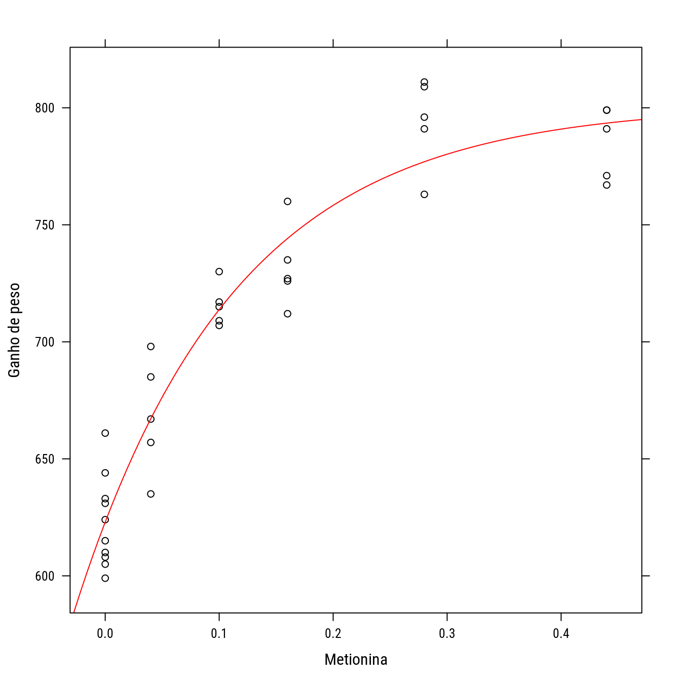
1.1 Configurações iniciais
#-----------------------------------------------------------------------
# Configurações iniciais.

packageVersion("acebayes")
## [1] '1.10'# Extremos do domínio da variável independente.
# dom <- range(turk0$A)
dom <- c(0, 0.6)
# Número pontos de suporte desejado.
# n_sup <- length(unique(turk0$A))
n_sup <- 10
# Delineamento regularmente espaçado para usar de valor inicial.
del_re <- cbind(A = seq(dom[1], dom[2], length.out = n_sup))
del_re## A
## [1,] 0.00000000
## [2,] 0.06666667
## [3,] 0.13333333
## [4,] 0.20000000
## [5,] 0.26666667
## [6,] 0.33333333
## [7,] 0.40000000
## [8,] 0.46666667
## [9,] 0.53333333
## [10,] 0.60000000p0 <- update(p0, xlim = extendrange(dom))
# Um delineamento equiespaçado.
p0 +
llayer(panel.abline(v = del_re, col = "gray"))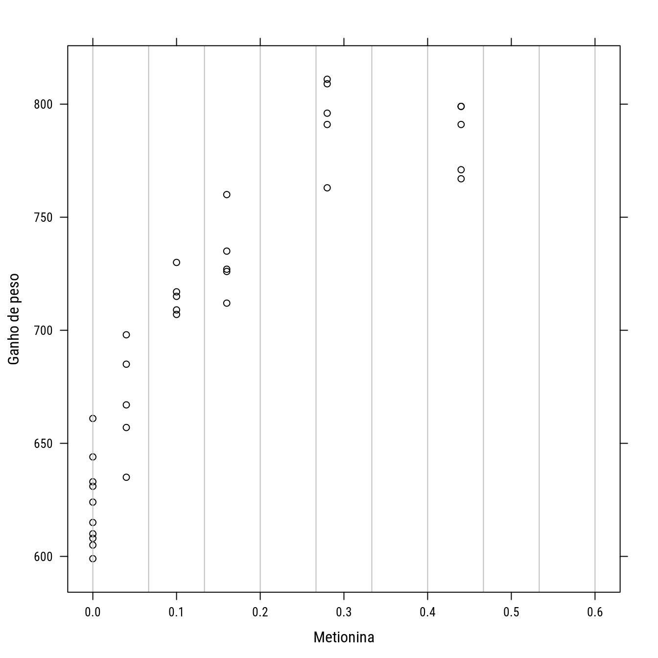
# Desenho inicial (v.a. uniforme).
start_d <- del_re
1.2 Delineamento ótimo Bayesiano com prioris uniformes
#-----------------------------------------------------------------------
# Priores uniformes para os parâmtros.

# Priores uniformes para os parâmetros.
prior_u <- list(support = cbind(f0 = c(0, 1000),
                                f1 = c(0, 1000),
                                k = c(0, 30)))

set.seed(1)
del_uni <- acenlm(formula = formula(n0)[-2],
                  start.d = start_d,
                  prior = prior_u,
                  criterion = "D",
                  N1 = 30,
                  N2 = 15,
                  lower = min(dom),
                  upper = max(dom),
                  progress = TRUE)
## Phase I iteration 1 out of 30 (Current value = 7.548787)
## Phase I iteration 2 out of 30 (Current value = 7.560806)
## Phase I iteration 3 out of 30 (Current value = 7.564025)
## Phase I iteration 4 out of 30 (Current value = 7.564515)
## Phase I iteration 5 out of 30 (Current value = 7.564517)
## Phase I iteration 6 out of 30 (Current value = 7.564517)
## Phase I iteration 7 out of 30 (Current value = 7.564517)
## Phase I iteration 8 out of 30 (Current value = 7.566358)
## Phase I iteration 9 out of 30 (Current value = 7.570033)
## Phase I iteration 10 out of 30 (Current value = 7.570033)
## Phase I iteration 11 out of 30 (Current value = 7.570033)
## Phase I iteration 12 out of 30 (Current value = 7.570033)
## Phase I iteration 13 out of 30 (Current value = 7.570034)
## Phase I iteration 14 out of 30 (Current value = 7.570034)
## Phase I iteration 15 out of 30 (Current value = 7.570034)
## Phase I iteration 16 out of 30 (Current value = 7.570034)
## Phase I iteration 17 out of 30 (Current value = 7.570034)
## Phase I iteration 18 out of 30 (Current value = 7.570034)
## Phase I iteration 19 out of 30 (Current value = 7.570068)
## Phase I iteration 20 out of 30 (Current value = 7.570068)
## Phase I iteration 21 out of 30 (Current value = 7.570068)
## Phase I iteration 22 out of 30 (Current value = 7.570068)
## Phase I iteration 23 out of 30 (Current value = 7.570068)
## Phase I iteration 24 out of 30 (Current value = 7.570068)
## Phase I iteration 25 out of 30 (Current value = 7.570068)
## Phase I iteration 26 out of 30 (Current value = 7.570068)
## Phase I iteration 27 out of 30 (Current value = 7.570068)
## Phase I iteration 28 out of 30 (Current value = 7.570068)
## Phase I iteration 29 out of 30 (Current value = 7.570068)
## Phase I iteration 30 out of 30 (Current value = 7.570068)
## Phase II iteration 1 out of 15 (Current value = 7.570068)
## Phase II iteration 2 out of 15 (Current value = 7.570068)
## Phase II iteration 3 out of 15 (Current value = 7.570068)
## Phase II iteration 4 out of 15 (Current value = 7.570068)
## Phase II iteration 5 out of 15 (Current value = 7.570068)
## Phase II iteration 6 out of 15 (Current value = 7.570068)
## Phase II iteration 7 out of 15 (Current value = 7.570068)
## Phase II iteration 8 out of 15 (Current value = 7.570068)
## Phase II iteration 9 out of 15 (Current value = 7.570068)
## Phase II iteration 10 out of 15 (Current value = 7.570068)
## Phase II iteration 11 out of 15 (Current value = 7.570068)
## Phase II iteration 12 out of 15 (Current value = 7.570068)
## Phase II iteration 13 out of 15 (Current value = 7.570068)
## Phase II iteration 14 out of 15 (Current value = 7.570068)
## Phase II iteration 15 out of 15 (Current value = 7.570068)summary(del_uni)## Non Linear Model
## Criterion = Bayesian D-optimality
## Formula: ~f0 + f1 * (1 - exp(-k * A))
## Method: quadrature
##
## nr = 2 , nq = 8
## Prior: uniform
##
## Number of runs = 10
##
## Number of factors = 1
##
## Number of Phase I iterations = 30
##
## Number of Phase II iterations = 15
##
## Computer time = 00:00:09# plot(del_uni)
# Resuldado para o delineamento ótimo.
cbind(phase1 = sort(del_uni$phase1.d),
phase2 = sort(del_uni$phase2.d))## phase1 phase2
## [1,] 0.00000000 0.00000000
## [2,] 0.00000000 0.00000000
## [3,] 0.00000000 0.00000000
## [4,] 0.05056983 0.05056983
## [5,] 0.05747182 0.05747182
## [6,] 0.05858971 0.05858971
## [7,] 0.25729415 0.25729415
## [8,] 0.60000000 0.60000000
## [9,] 0.60000000 0.60000000
## [10,] 0.60000000 0.60000000table(round(del_uni$phase2.d, digits = 2))##
## 0 0.05 0.06 0.26 0.6
## 3 1 2 1 3p0 +
llayer(panel.abline(v = del_uni$phase2.d, col = "orange"))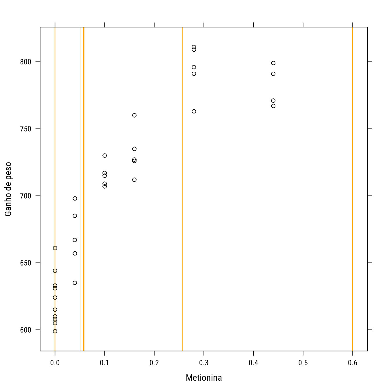
1.3 Delimeanto ótimo Bayesiano com prioris Gaussianas
#-----------------------------------------------------------------------
# Priores gaussianas com método de Monte Carlo.

prior_g <- list(mu = c(f0 = 500, f1 = 200, k = 10),
                sigma2 = c(f0 = 200^2, f1 = 100^2, k = 3^2))

del_gau <- acenlm(formula = formula(n0)[-2],
                  start.d = start_d,
                  prior = prior_g,
                  criterion = "D",
                  N1 = 30,
                  N2 = 15,
                  lower = min(dom),
                  upper = max(dom),
                  progress = TRUE)
## Phase I iteration 1 out of 30 (Current value = 7.000296)
## Phase I iteration 2 out of 30 (Current value = 7.100751)
## Phase I iteration 3 out of 30 (Current value = 7.10128)
## Phase I iteration 4 out of 30 (Current value = 7.10128)
## Phase I iteration 5 out of 30 (Current value = 7.10128)
## Phase I iteration 6 out of 30 (Current value = 7.101291)
## Phase I iteration 7 out of 30 (Current value = 7.101291)
## Phase I iteration 8 out of 30 (Current value = 7.10133)
## Phase I iteration 9 out of 30 (Current value = 7.101349)
## Phase I iteration 10 out of 30 (Current value = 7.101358)
## Phase I iteration 11 out of 30 (Current value = 7.101358)
## Phase I iteration 12 out of 30 (Current value = 7.10136)
## Phase I iteration 13 out of 30 (Current value = 7.101361)
## Phase I iteration 14 out of 30 (Current value = 7.101361)
## Phase I iteration 15 out of 30 (Current value = 7.101362)
## Phase I iteration 16 out of 30 (Current value = 7.101362)
## Phase I iteration 17 out of 30 (Current value = 7.101363)
## Phase I iteration 18 out of 30 (Current value = 7.101363)
## Phase I iteration 19 out of 30 (Current value = 7.101363)
## Phase I iteration 20 out of 30 (Current value = 7.101363)
## Phase I iteration 21 out of 30 (Current value = 7.101363)
## Phase I iteration 22 out of 30 (Current value = 7.101363)
## Phase I iteration 23 out of 30 (Current value = 7.101363)
## Phase I iteration 24 out of 30 (Current value = 7.101363)
## Phase I iteration 25 out of 30 (Current value = 7.101365)
## Phase I iteration 26 out of 30 (Current value = 7.101365)
## Phase I iteration 27 out of 30 (Current value = 7.101365)
## Phase I iteration 28 out of 30 (Current value = 7.101365)
## Phase I iteration 29 out of 30 (Current value = 7.101366)
## Phase I iteration 30 out of 30 (Current value = 7.101366)
## Phase II iteration 1 out of 15 (Current value = 7.101368)
## Phase II iteration 2 out of 15 (Current value = 7.101368)
## Phase II iteration 3 out of 15 (Current value = 7.101368)
## Phase II iteration 4 out of 15 (Current value = 7.101368)
## Phase II iteration 5 out of 15 (Current value = 7.101368)
## Phase II iteration 6 out of 15 (Current value = 7.101368)
## Phase II iteration 7 out of 15 (Current value = 7.101368)
## Phase II iteration 8 out of 15 (Current value = 7.101368)
## Phase II iteration 9 out of 15 (Current value = 7.101368)
## Phase II iteration 10 out of 15 (Current value = 7.101368)
## Phase II iteration 11 out of 15 (Current value = 7.101368)
## Phase II iteration 12 out of 15 (Current value = 7.101368)
## Phase II iteration 13 out of 15 (Current value = 7.101368)
## Phase II iteration 14 out of 15 (Current value = 7.101368)
## Phase II iteration 15 out of 15 (Current value = 7.101368)summary(del_gau)## Non Linear Model
## Criterion = Bayesian D-optimality
## Formula: ~f0 + f1 * (1 - exp(-k * A))
## Method: quadrature
##
## nr = 2 , nq = 8
## Prior: normal
##
## Number of runs = 10
##
## Number of factors = 1
##
## Number of Phase I iterations = 30
##
## Number of Phase II iterations = 15
##
## Computer time = 00:00:09# plot(del_gau)
# Resuldado para o delineamento ótimo.
cbind(phase1 = sort(del_gau$phase1.d),
phase2 = sort(del_gau$phase2.d))## phase1 phase2
## [1,] 0.00000000 0.00000000
## [2,] 0.00000000 0.00000000
## [3,] 0.00000000 0.00000000
## [4,] 0.09775279 0.09777919
## [5,] 0.09777919 0.09777919
## [6,] 0.09783794 0.09783794
## [7,] 0.09820545 0.09783794
## [8,] 0.60000000 0.60000000
## [9,] 0.60000000 0.60000000
## [10,] 0.60000000 0.60000000table(round(del_gau$phase2.d, digits = 2))##
## 0 0.1 0.6
## 3 4 3p0 +
llayer(panel.abline(v = del_gau$phase2.d, col = "orange"))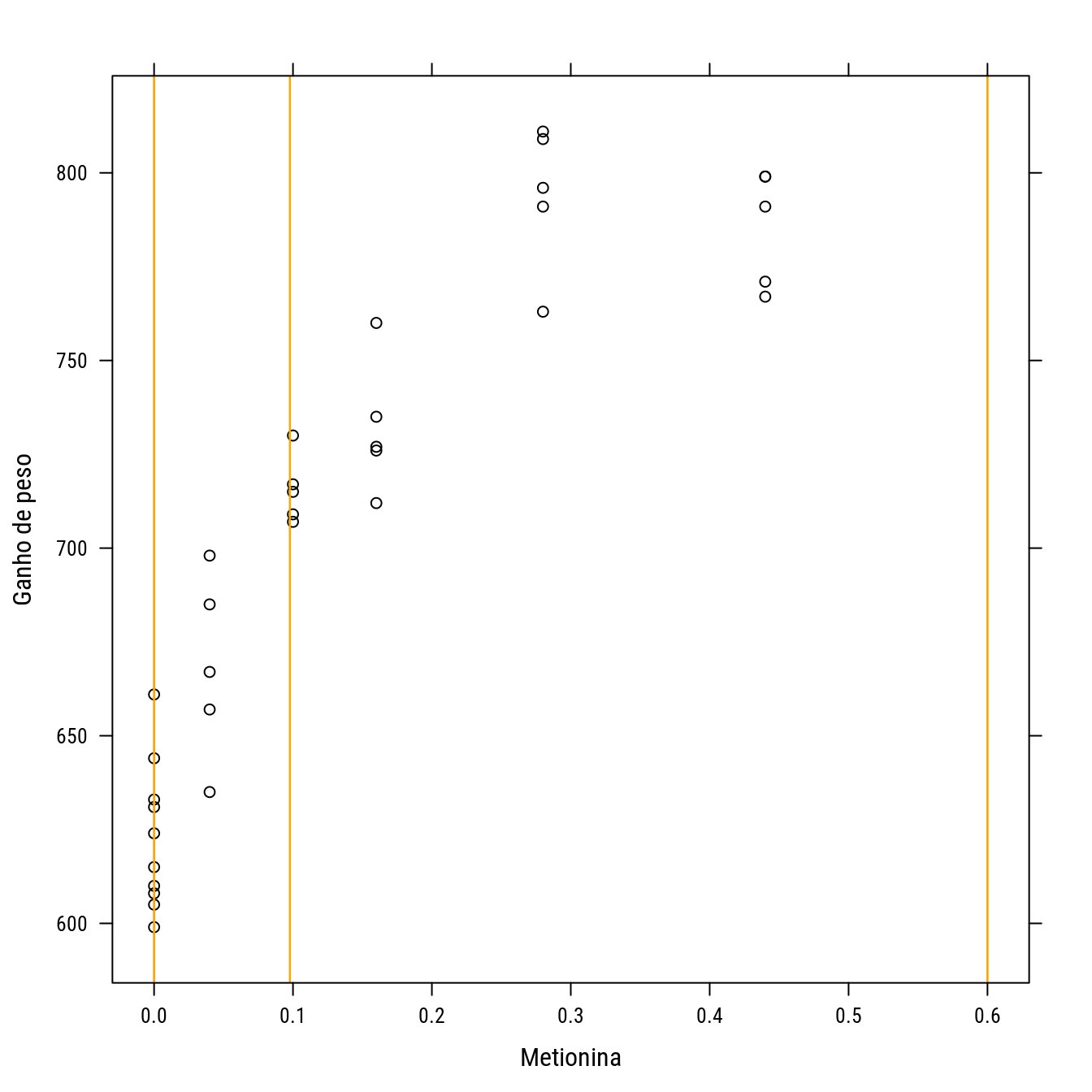
1.4 Delimeanto ótimo Bayesiano com prioris uniformes e restrição
O deliamento a seguir preserva as configurações anteriores. No entanto, é incluída a restrição de que os pontos de suporte consecutivos devem estar espaçadas de pelo menos algumas unidades.
# Fornece a restrição de espaçamento mínimo.

# Se usar o valor abaixo, vai forçar um delineamento equiespaçado.
min_dist <- diff(range(dom))/(nrow(del_re) - 1)
min_dist
## [1] 0.06666667# seq(dom[1], dom[2], by = min_dist)
# Usar uma fração então.
min_dist <- min_dist/4
limits <- function(d, i, j) {
grid <- seq(from = dom[1], to = dom[2], length.out = 1000)
for (s in as.vector(d)[-i]) {
cond <- (grid <= (s - min_dist)) | (grid >= (s + min_dist))
grid <- grid[cond]
}
return(grid)
}del_uni_lim <- acenlm(formula = formula(n0)[-2],
start.d = start_d,
prior = prior_u,
criterion = "D",
N1 = 30,
N2 = 15,
limits = limits,
lower = min(dom),
upper = max(dom),
progress = TRUE)## Phase I iteration 1 out of 30 (Current value = 7.137992)
## Phase I iteration 2 out of 30 (Current value = 7.138438)
## Phase I iteration 3 out of 30 (Current value = 7.140948)
## Phase I iteration 4 out of 30 (Current value = 7.14098)
## Phase I iteration 5 out of 30 (Current value = 7.14098)
## Phase I iteration 6 out of 30 (Current value = 7.14098)
## Phase I iteration 7 out of 30 (Current value = 7.14098)
## Phase I iteration 8 out of 30 (Current value = 7.14098)
## Phase I iteration 9 out of 30 (Current value = 7.14098)
## Phase I iteration 10 out of 30 (Current value = 7.140994)
## Phase I iteration 11 out of 30 (Current value = 7.140994)
## Phase I iteration 12 out of 30 (Current value = 7.140994)
## Phase I iteration 13 out of 30 (Current value = 7.140994)
## Phase I iteration 14 out of 30 (Current value = 7.140994)
## Phase I iteration 15 out of 30 (Current value = 7.140994)
## Phase I iteration 16 out of 30 (Current value = 7.140994)
## Phase I iteration 17 out of 30 (Current value = 7.140994)
## Phase I iteration 18 out of 30 (Current value = 7.140994)
## Phase I iteration 19 out of 30 (Current value = 7.140994)
## Phase I iteration 20 out of 30 (Current value = 7.140994)
## Phase I iteration 21 out of 30 (Current value = 7.140994)
## Phase I iteration 22 out of 30 (Current value = 7.140994)
## Phase I iteration 23 out of 30 (Current value = 7.140994)
## Phase I iteration 24 out of 30 (Current value = 7.140994)
## Phase I iteration 25 out of 30 (Current value = 7.140994)
## Phase I iteration 26 out of 30 (Current value = 7.140994)
## Phase I iteration 27 out of 30 (Current value = 7.140994)
## Phase I iteration 28 out of 30 (Current value = 7.140994)
## Phase I iteration 29 out of 30 (Current value = 7.140994)
## Phase I iteration 30 out of 30 (Current value = 7.140994)
## Phase II iteration 1 out of 15 (Current value = 7.41237)
## Phase II iteration 2 out of 15 (Current value = 7.535847)
## Phase II iteration 3 out of 15 (Current value = 7.535847)
## Phase II iteration 4 out of 15 (Current value = 7.535847)
## Phase II iteration 5 out of 15 (Current value = 7.535847)
## Phase II iteration 6 out of 15 (Current value = 7.535847)
## Phase II iteration 7 out of 15 (Current value = 7.535847)
## Phase II iteration 8 out of 15 (Current value = 7.535847)
## Phase II iteration 9 out of 15 (Current value = 7.535847)
## Phase II iteration 10 out of 15 (Current value = 7.535847)
## Phase II iteration 11 out of 15 (Current value = 7.535847)
## Phase II iteration 12 out of 15 (Current value = 7.535847)
## Phase II iteration 13 out of 15 (Current value = 7.535847)
## Phase II iteration 14 out of 15 (Current value = 7.535847)
## Phase II iteration 15 out of 15 (Current value = 7.535847)del_uni_lim## Non Linear Model
## Criterion = Bayesian D-optimality
## Formula: ~f0 + f1 * (1 - exp(-k * A))
## Method: quadrature
##
## nr = 2 , nq = 8
## Prior: uniform
##
## Number of runs = 10
##
## Number of factors = 1
##
## Number of Phase I iterations = 30
##
## Number of Phase II iterations = 15
##
## Computer time = 00:00:08summary(del_uni_lim)## Non Linear Model
## Criterion = Bayesian D-optimality
## Formula: ~f0 + f1 * (1 - exp(-k * A))
## Method: quadrature
##
## nr = 2 , nq = 8
## Prior: uniform
##
## Number of runs = 10
##
## Number of factors = 1
##
## Number of Phase I iterations = 30
##
## Number of Phase II iterations = 15
##
## Computer time = 00:00:08# plot(del_uni_lim)
# Resuldado para o delineamento ótimo.
cbind(phase1 = sort(del_uni_lim$phase1.d),
phase2 = sort(del_uni_lim$phase2.d))## phase1 phase2
## [1,] 0.00000000 0.00000000
## [2,] 0.01681682 0.00000000
## [3,] 0.04444444 0.00000000
## [4,] 0.06126126 0.04444444
## [5,] 0.07807808 0.06126126
## [6,] 0.24744745 0.07807808
## [7,] 0.26426426 0.26426426
## [8,] 0.56636637 0.56636637
## [9,] 0.58318318 0.58318318
## [10,] 0.60000000 0.60000000table(round(del_uni_lim$phase1.d, digits = 2))##
## 0 0.02 0.04 0.06 0.08 0.25 0.26 0.57 0.58 0.6
## 1 1 1 1 1 1 1 1 1 1p0 +
llayer(panel.abline(v = del_uni_lim$phase1.d, col = "orange"))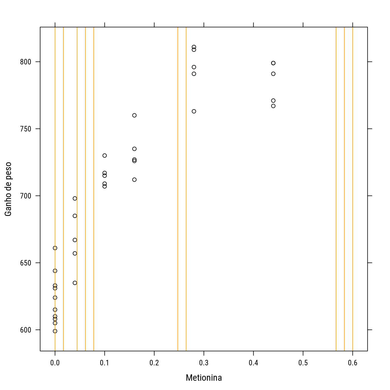
1.5 Delimeanto ótimo Bayesiano com prioris Gaussianas e restrição
del_gau_lim <- acenlm(formula = formula(n0)[-2],
                      start.d = start_d,
                      prior = prior_g,
                      criterion = "D",
                      N1 = 30,
                      N2 = 15,
                      limits = limits,
                      lower = min(dom),
                      upper = max(dom),
                      progress = TRUE)
## Phase I iteration 1 out of 30 (Current value = 6.617585)
## Phase I iteration 2 out of 30 (Current value = 6.690034)
## Phase I iteration 3 out of 30 (Current value = 6.690034)
## Phase I iteration 4 out of 30 (Current value = 6.690034)
## Phase I iteration 5 out of 30 (Current value = 6.690034)
## Phase I iteration 6 out of 30 (Current value = 6.690034)
## Phase I iteration 7 out of 30 (Current value = 6.690034)
## Phase I iteration 8 out of 30 (Current value = 6.690034)
## Phase I iteration 9 out of 30 (Current value = 6.690034)
## Phase I iteration 10 out of 30 (Current value = 6.690034)
## Phase I iteration 11 out of 30 (Current value = 6.690034)
## Phase I iteration 12 out of 30 (Current value = 6.690034)
## Phase I iteration 13 out of 30 (Current value = 6.690034)
## Phase I iteration 14 out of 30 (Current value = 6.690034)
## Phase I iteration 15 out of 30 (Current value = 6.690034)
## Phase I iteration 16 out of 30 (Current value = 6.690034)
## Phase I iteration 17 out of 30 (Current value = 6.690034)
## Phase I iteration 18 out of 30 (Current value = 6.690034)
## Phase I iteration 19 out of 30 (Current value = 6.690034)
## Phase I iteration 20 out of 30 (Current value = 6.690034)
## Phase I iteration 21 out of 30 (Current value = 6.690034)
## Phase I iteration 22 out of 30 (Current value = 6.690034)
## Phase I iteration 23 out of 30 (Current value = 6.690034)
## Phase I iteration 24 out of 30 (Current value = 6.690034)
## Phase I iteration 25 out of 30 (Current value = 6.690034)
## Phase I iteration 26 out of 30 (Current value = 6.690034)
## Phase I iteration 27 out of 30 (Current value = 6.690034)
## Phase I iteration 28 out of 30 (Current value = 6.690034)
## Phase I iteration 29 out of 30 (Current value = 6.690034)
## Phase I iteration 30 out of 30 (Current value = 6.690034)
## Phase II iteration 1 out of 15 (Current value = 6.947997)
## Phase II iteration 2 out of 15 (Current value = 7.071785)
## Phase II iteration 3 out of 15 (Current value = 7.081054)
## Phase II iteration 4 out of 15 (Current value = 7.085449)
## Phase II iteration 5 out of 15 (Current value = 7.087346)
## Phase II iteration 6 out of 15 (Current value = 7.09761)
## Phase II iteration 7 out of 15 (Current value = 7.100029)
## Phase II iteration 8 out of 15 (Current value = 7.100029)
## Phase II iteration 9 out of 15 (Current value = 7.100029)
## Phase II iteration 10 out of 15 (Current value = 7.100029)
## Phase II iteration 11 out of 15 (Current value = 7.100029)
## Phase II iteration 12 out of 15 (Current value = 7.100029)
## Phase II iteration 13 out of 15 (Current value = 7.100029)
## Phase II iteration 14 out of 15 (Current value = 7.100029)
## Phase II iteration 15 out of 15 (Current value = 7.100029)summary(del_gau_lim)## Non Linear Model
## Criterion = Bayesian D-optimality
## Formula: ~f0 + f1 * (1 - exp(-k * A))
## Method: quadrature
##
## nr = 2 , nq = 8
## Prior: normal
##
## Number of runs = 10
##
## Number of factors = 1
##
## Number of Phase I iterations = 30
##
## Number of Phase II iterations = 15
##
## Computer time = 00:00:08# plot(del_gau_lim)
# Resuldado para o delineamento ótimo.
cbind(phase1 = sort(del_gau_lim$phase1.d),
phase2 = sort(del_gau_lim$phase2.d))## phase1 phase2
## [1,] 0.00000000 0.00000000
## [2,] 0.01681682 0.00000000
## [3,] 0.07747748 0.00000000
## [4,] 0.09429429 0.09429429
## [5,] 0.11111111 0.09429429
## [6,] 0.12792793 0.09429429
## [7,] 0.54954955 0.60000000
## [8,] 0.56636637 0.60000000
## [9,] 0.58318318 0.60000000
## [10,] 0.60000000 0.60000000table(round(del_gau_lim$phase1.d, digits = 2))##
## 0 0.02 0.08 0.09 0.11 0.13 0.55 0.57 0.58 0.6
## 1 1 1 1 1 1 1 1 1 1p0 +
llayer(panel.abline(v = del_gau_lim$phase1.d, col = "orange"))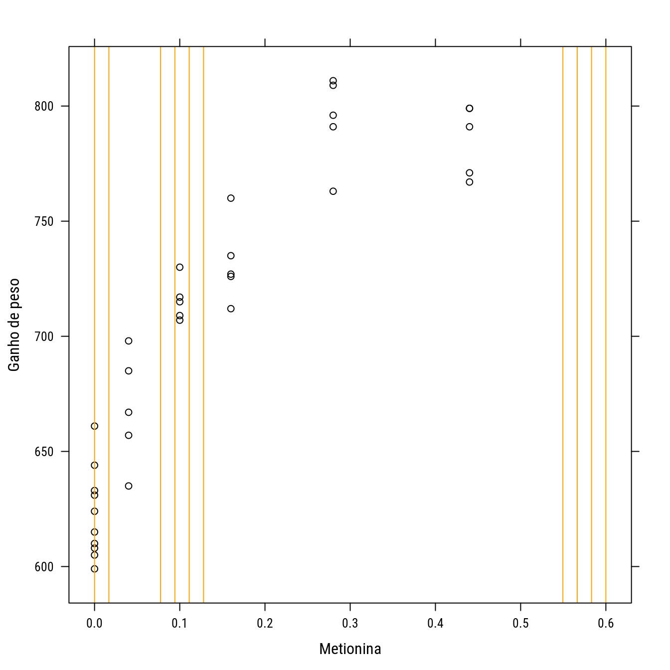
1.6 Comparação dos resultados
#-----------------------------------------------------------------------
# Resumo.

# Delineamentos bayesianos obtidos.
del_baye <- list(del_uni,
                 del_uni_lim,
                 del_gau,
                 del_gau_lim)
names(del_baye) <- c("U", "UR", "N", "NR")

del_sup <- lapply(del_baye, FUN = "[[", "phase1.d")
# del_sup

# Tabela com os pontos de suporte de cada delineamento.
tb_del <- lapply(del_sup, FUN = as.vector)
tb_del <- lapply(tb_del, FUN = sort)
tb_del <- do.call(cbind, tb_del)
tb_del
## U UR N NR
## [1,] 0.00000000 0.00000000 0.00000000 0.00000000
## [2,] 0.00000000 0.01681682 0.00000000 0.01681682
## [3,] 0.00000000 0.04444444 0.00000000 0.07747748
## [4,] 0.05056983 0.06126126 0.09775279 0.09429429
## [5,] 0.05747182 0.07807808 0.09777919 0.11111111
## [6,] 0.05858971 0.24744745 0.09783794 0.12792793
## [7,] 0.25729415 0.26426426 0.09820545 0.54954955
## [8,] 0.60000000 0.56636637 0.60000000 0.56636637
## [9,] 0.60000000 0.58318318 0.60000000 0.58318318
## [10,] 0.60000000 0.60000000 0.60000000 0.60000000#-----------------------------------------------------------------------
# Obtenção das eficiências relativas com relação aos delineamento
# Bayesianos.
# Eficiencias absolutas.
util <- sapply(del_baye,
FUN = function(del) {
del$utility(del$phase1.d)
})
sort(util)## NR N UR U
## 6.690034 7.101366 7.140994 7.570068# Amplitude de variação em eficiência absoluta.
range(util)## [1] 6.690034 7.570068# Melhor e pior delineamento.
del_baye[[which.max(util)]]## Non Linear Model
## Criterion = Bayesian D-optimality
## Formula: ~f0 + f1 * (1 - exp(-k * A))
## Method: quadrature
##
## nr = 2 , nq = 8
## Prior: uniform
##
## Number of runs = 10
##
## Number of factors = 1
##
## Number of Phase I iterations = 30
##
## Number of Phase II iterations = 15
##
## Computer time = 00:00:09del_baye[[which.min(util)]]## Non Linear Model
## Criterion = Bayesian D-optimality
## Formula: ~f0 + f1 * (1 - exp(-k * A))
## Method: quadrature
##
## nr = 2 , nq = 8
## Prior: normal
##
## Number of runs = 10
##
## Number of factors = 1
##
## Number of Phase I iterations = 30
##
## Number of Phase II iterations = 15
##
## Computer time = 00:00:08# Compara os delineamentos mais contrastantes.
assess(d1 = del_baye[[which.max(util)]],
d2 = del_baye[[which.min(util)]])## Approximate expected utility of d1 = 7.570068
## Approximate expected utility of d2 = 7.302126
## Approximate relative D-efficiency = 109.3424%del_baye[[which.max(util)]]$phase1d## NULL|
Modelos de Regressão Não Linear: Fundamentos e Aplicações em R leg.ufpr.br/~walmes/cursoR/mrnl |
Prof. Walmes M. Zeviani Departamento de Estatística · UFPR |