|
|
Modelos de Regressão Não LinearFundamentos e Aplicações em R |
Ajuste de modelos não lineares considerando estrutura experimental
- http://leg.ufpr.br/~walmes/analises/HSSDuarte/curva-progresso.html.
- http://leg.ufpr.br/~walmes/analises/MESerafim/abacaxi/abacaxicra.html.
- http://leg.ufpr.br/~walmes/pacotes/EACS/articles/maracuja.html#crescimento-das-plantas-via-modelo-nao-linear-de-efeitos-aleatorios.
- http://leg.ufpr.br/~walmes/pacotes/RDASC/articles/leaf_spot.html.
1 Desfolha do algodão
library(latticeExtra)
library(nlme)

llayer <- latticeExtra::layer
source("https://raw.githubusercontent.com/walmes/wzRfun/master/R/panel.cbH.R")
#-----------------------------------------------------------------------
# Dados de peso de capulhos de algodão em função do nível de desfilha
# artificial.
cap <- read.table("http://www.leg.ufpr.br/~walmes/data/algodão.txt",
header = TRUE, sep = "\t", encoding = "latin1")
cap <- transform(cap,
desf = desf/100,
estag = factor(estag))
str(cap)## 'data.frame': 125 obs. of 8 variables:
## $ estag : Factor w/ 5 levels "1veg","2bot",..: 1 1 1 1 1 1 1 1 1 1 ...
## $ desf : num 0 0 0 0 0 0.25 0.25 0.25 0.25 0.25 ...
## $ rep : int 1 2 3 4 5 1 2 3 4 5 ...
## $ pcapu : num 33.2 28.7 31.5 28.9 36.4 ...
## $ nnos : int 32 29 29 27 28 30 33 23 29 26 ...
## $ alt : num 151 146 140 155 150 ...
## $ ncapu : int 10 9 8 8 10 11 9 10 10 10 ...
## $ nestru: int 10 9 8 9 10 11 9 11 10 10 ...estagios <- c("Vegetativo", "Botão floral", "Florescimento", "Maçã",
"Capulho")
#-----------------------------------------------------------------------
# Ajuste dos modelos separados por um fator categórico.
p0 <-
xyplot(pcapu ~ desf | estag,
data = cap,
layout = c(NA, 2),
as.table = TRUE,
xlab = "Nível de desfolha artificial",
ylab = "Peso de capulhos")
p0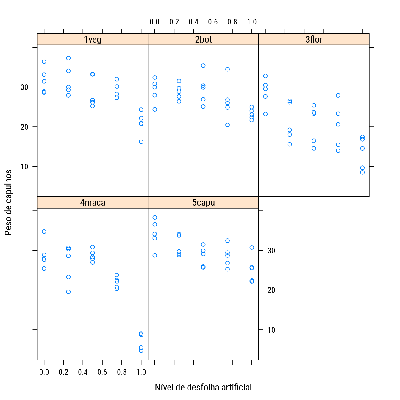
# ~f0 - f1 * desf^((log(5) - log(f1))/log(xde))
# ~f0 - f1 * desf^exp(curv)

# A `nlsList()` é basicamente a `nls()` dentro de um `lapply()`.
n00 <- nlsList(pcapu ~ f0 - f1 *
                   desf^((log(5) - log(f1))/log(xde)) | estag,
               data = cap,
               start = c(f0 = 30, f1 = 8, xde = 0.8))
coef(n00)
## f0 f1 xde
## 1veg 31.14929 10.166278 0.8538319
## 2bot 29.26289 6.117394 0.9440160
## 3flor 28.50115 13.014666 0.2021585
## 4maça 28.26343 21.608571 0.7243578
## 5capu 34.15315 8.277792 0.4954646# Como prover valores iniciais a partir deste ajuste.
L <- cbind(1, contrasts(cap$estag))
L## 2bot 3flor 4maça 5capu
## 1veg 1 0 0 0 0
## 2bot 1 1 0 0 0
## 3flor 1 0 1 0 0
## 4maça 1 0 0 1 0
## 5capu 1 0 0 0 1# \mu = L \beta, então \beta = L^{-1} \mu.
start <- solve(L) %*% as.matrix(coef(n00))
c(start)## [1] 31.14929457 -1.88640219 -2.64814939 -2.88586070 3.00385297 10.16627822 -4.04888413
## [8] 2.84838777 11.44229229 -1.88848629 0.85383191 0.09018408 -0.65167345 -0.12947410
## [15] -0.35836736#-----------------------------------------------------------------------
# Ajuste conjunto.
n0 <- gnls(model = pcapu ~ f0 - f1 * desf^((log(5) - log(f1))/log(xde)),
params = f0 + f1 + xde ~ estag,
# start = c(30, 0, 0, 0, 0,
# 8, 0, 0, 0, 0,
# 0.1, 0, 0, 0, 0),
start = c(start),
data = cap)
summary(n0)## Generalized nonlinear least squares fit
## Model: pcapu ~ f0 - f1 * desf^((log(5) - log(f1))/log(xde))
## Data: cap
## AIC BIC logLik
## 687.3049 732.5579 -327.6524
##
## Coefficients:
## Value Std.Error t-value p-value
## f0.(Intercept) 31.149266 1.0413031 29.913735 0.0000
## f0.estag2bot -1.886383 1.5260306 -1.236137 0.2190
## f0.estag3flor -2.648075 1.8939030 -1.398211 0.1649
## f0.estag4maça -2.885844 1.4707311 -1.962183 0.0523
## f0.estag5capu 3.003895 1.8900426 1.589327 0.1149
## f1.(Intercept) 10.166268 1.8711175 5.433260 0.0000
## f1.estag2bot -4.048876 2.6572896 -1.523687 0.1305
## f1.estag3flor 2.848397 2.7639130 1.030567 0.3050
## f1.estag4maça 11.442298 2.6457253 4.324825 0.0000
## f1.estag5capu -1.888474 2.7631564 -0.683448 0.4958
## xde.(Intercept) 0.853835 0.0809136 10.552434 0.0000
## xde.estag2bot 0.090181 0.1268542 0.710905 0.4786
## xde.estag3flor -0.651684 0.1549329 -4.206236 0.0001
## xde.estag4maça -0.129476 0.1005280 -1.287964 0.2005
## xde.estag5capu -0.358374 0.2776476 -1.290752 0.1995
##
## Correlation:
## f0.(I) f0.st2 f0.st3 f0st4ç f0.st5 f1.(I) f1.st2 f1.st3 f1st4ç f1.st5
## f0.estag2bot -0.682
## f0.estag3flor -0.550 0.375
## f0.estag4maça -0.708 0.483 0.389
## f0.estag5capu -0.551 0.376 0.303 0.390
## f1.(Intercept) 0.533 -0.363 -0.293 -0.377 -0.293
## f1.estag2bot -0.375 0.541 0.206 0.266 0.207 -0.704
## f1.estag3flor -0.361 0.246 0.661 0.255 0.199 -0.677 0.477
## f1.estag4maça -0.377 0.257 0.207 0.532 0.208 -0.707 0.498 0.479
## f1.estag5capu -0.361 0.246 0.198 0.255 0.654 -0.677 0.477 0.458 0.479
## xde.(Intercept) -0.708 0.483 0.389 0.501 0.390 -0.530 0.373 0.359 0.375 0.359
## xde.estag2bot 0.452 -0.721 -0.248 -0.320 -0.249 0.338 -0.728 -0.229 -0.239 -0.229
## xde.estag3flor 0.370 -0.252 -0.730 -0.262 -0.204 0.277 -0.195 -0.434 -0.196 -0.187
## xde.estag4maça 0.570 -0.389 -0.313 -0.677 -0.314 0.427 -0.300 -0.289 -0.445 -0.289
## xde.estag5capu 0.206 -0.141 -0.113 -0.146 -0.806 0.154 -0.109 -0.105 -0.109 -0.576
## xd.(I) xd.st2 xd.st3 xdst4ç
## f0.estag2bot
## f0.estag3flor
## f0.estag4maça
## f0.estag5capu
## f1.(Intercept)
## f1.estag2bot
## f1.estag3flor
## f1.estag4maça
## f1.estag5capu
## xde.(Intercept)
## xde.estag2bot -0.638
## xde.estag3flor -0.522 0.333
## xde.estag4maça -0.805 0.513 0.420
## xde.estag5capu -0.291 0.186 0.152 0.235
##
## Standardized residuals:
## Min Q1 Med Q3 Max
## -2.43631478 -0.59093061 -0.03534145 0.60230115 2.92708061
##
## Residual standard error: 3.547339
## Degrees of freedom: 125 total; 110 residual# Estimativas dos parâmetros.
matrix(kronecker(diag(3), L) %*% cbind(coef(n0)),
ncol = ncol(coef(n00)))## [,1] [,2] [,3]
## [1,] 31.14927 10.166268 0.8538355
## [2,] 29.26288 6.117391 0.9440167
## [3,] 28.50119 13.014665 0.2021511
## [4,] 28.26342 21.608566 0.7243590
## [5,] 34.15316 8.277793 0.4954611coef(n00)## f0 f1 xde
## 1veg 31.14929 10.166278 0.8538319
## 2bot 29.26289 6.117394 0.9440160
## 3flor 28.50115 13.014666 0.2021585
## 4maça 28.26343 21.608571 0.7243578
## 5capu 34.15315 8.277792 0.4954646# Quadros de testes de Wald.
anova(n0, type = "sequential")## Denom. DF: 110
## numDF F-value p-value
## f0.(Intercept) 1 13064.520 <.0001
## f0.estag 4 124.019 <.0001
## f1.(Intercept) 1 1355.491 <.0001
## f1.estag 4 23.604 <.0001
## xde.(Intercept) 1 379.711 <.0001
## xde.estag 4 6.769 1e-04anova(n0, type = "marginal")## Denom. DF: 110
## numDF F-value p-value
## f0.(Intercept) 1 1016.8540 <.0001
## f0.estag 4 3.4885 0.0101
## f1.(Intercept) 1 33.5458 <.0001
## f1.estag 4 11.5520 <.0001
## xde.(Intercept) 1 126.5385 <.0001
## xde.estag 4 6.7691 0.0001#-----------------------------------------------------------------------
# Vendo o ajuste.
pred <- expand.grid(desf = seq(0, 1, length.out = 30),
estag = levels(cap$estag))
pred$y <- predict(n0, newdata = pred)
p0 +
as.layer(xyplot(y ~ desf | estag,
data = pred,
type = "l",
col = 1))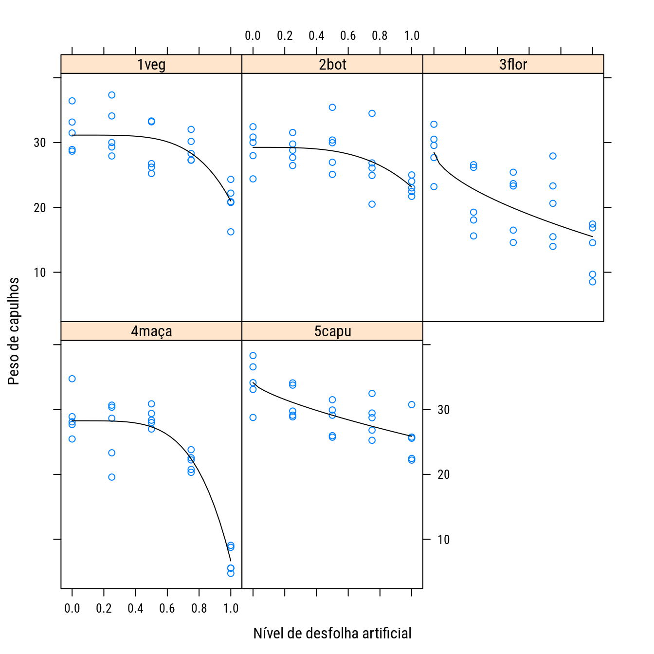
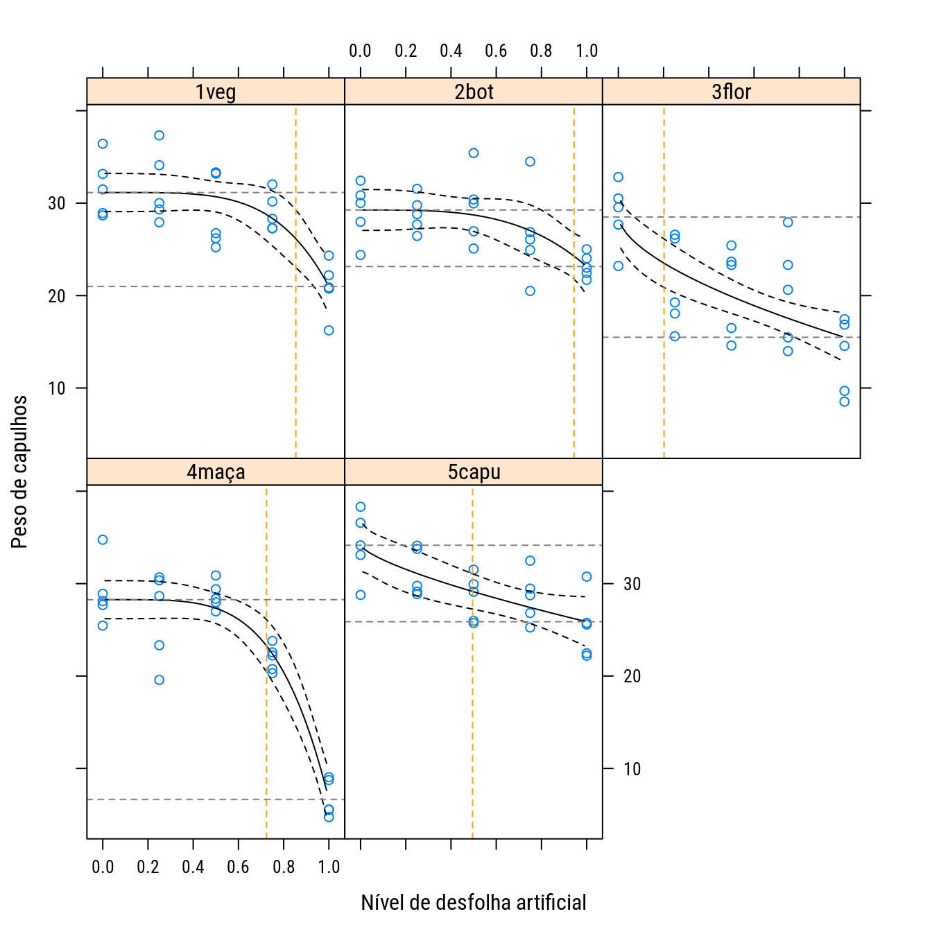
#-----------------------------------------------------------------------
# Bandas de confiança.

# Ajuste do modelo com a parametrização de estimativas por nível.
n1 <- gnls(model = pcapu ~ f0 - f1 * desf^((log(5) - log(f1))/log(xde)),
           params = f0 + f1 + xde ~ 0 + estag,
           start = unlist(coef(n00)),
           data = cap)
coef(n1)
## f0.estag1veg f0.estag2bot f0.estag3flor f0.estag4maça f0.estag5capu f1.estag1veg
## 31.1492661 29.2628832 28.5011909 28.2634222 34.1531614 10.1662677
## f1.estag2bot f1.estag3flor f1.estag4maça f1.estag5capu xde.estag1veg xde.estag2bot
## 6.1173915 13.0146650 21.6085661 8.2777934 0.8538355 0.9440167
## xde.estag3flor xde.estag4maça xde.estag5capu
## 0.2021511 0.7243590 0.4954611# Verifica que a medida de ajuste é a mesma.
logLik(n0)## 'log Lik.' -327.6524 (df=16)logLik(n1)## 'log Lik.' -327.6524 (df=16)# Retorna f(x, theta), f'(x, theta) e f''(x, theta).
model <- deriv3(expr = ~f0 - f1 * x^((log(5) - log(f1))/log(xde)),
namevec = c("f0", "f1", "xde"),
function.arg = function(x, f0, f1, xde) {
NULL
})
# Obtendo a matriz do modelo: derivadas parciais em theta avaliados em
# cada x_i.
# Obtendo os componentes para um vetor x e valores dos parâmetros.
model(x = c(0.1, 0.5, 0.9), f0 = 30, f1 = 8, xde = 0.5)## [1] 28.32113 25.00000 22.55160
## attr(,"gradient")
## f0 f1 xde
## [1,] 1 0.4872781 7.563348
## [2,] 1 0.0000000 6.780719
## [3,] 1 -0.7895278 1.535399
## attr(,"hessian")
## , , f0
##
## f0 f1 xde
## [1,] 0 0 0
## [2,] 0 0 0
## [3,] 0 0 0
##
## , , f1
##
## f0 f1 xde
## [1,] 0 -0.20233784 -0.1836806
## [2,] 0 0.00000000 1.8033688
## [3,] 0 0.01500133 0.5710994
##
## , , xde
##
## f0 f1 xde
## [1,] 0 -0.1836806 -5.553252
## [2,] 0 1.8033688 16.372971
## [3,] 0 0.5710994 5.473148# Grid de valores para predição com bandas.
desf.seq <- seq(0.01, 0.99, length.out = 41)
pred <- expand.grid(desf = desf.seq,
estag = levels(cap$estag),
KEEP.OUT.ATTRS = FALSE)
pred$y <- predict(n1, newdata = pred)
# Cria lista com as estimativas de cada nível separadas.
s <- sub("^.*\\.", "", x = names(coef(n1)))
ths <- split(coef(n1), s)
ths## $estag1veg
## f0.estag1veg f1.estag1veg xde.estag1veg
## 31.1492661 10.1662677 0.8538355
##
## $estag2bot
## f0.estag2bot f1.estag2bot xde.estag2bot
## 29.2628832 6.1173915 0.9440167
##
## $estag3flor
## f0.estag3flor f1.estag3flor xde.estag3flor
## 28.5011909 13.0146650 0.2021511
##
## $estag4maça
## f0.estag4maça f1.estag4maça xde.estag4maça
## 28.263422 21.608566 0.724359
##
## $estag5capu
## f0.estag5capu f1.estag5capu xde.estag5capu
## 34.1531614 8.2777934 0.4954611# Acerta os nomes.
ths <- lapply(ths, "names<-", c("f0", "f1", "xde"))
ths## $estag1veg
## f0 f1 xde
## 31.1492661 10.1662677 0.8538355
##
## $estag2bot
## f0 f1 xde
## 29.2628832 6.1173915 0.9440167
##
## $estag3flor
## f0 f1 xde
## 28.5011909 13.0146650 0.2021511
##
## $estag4maça
## f0 f1 xde
## 28.263422 21.608566 0.724359
##
## $estag5capu
## f0 f1 xde
## 34.1531614 8.2777934 0.4954611i <- 0
mm <- lapply(ths,
FUN = function(th) {
i <<- i + 1
d3 <- do.call(what = model,
args = c(list(x = desf.seq),
as.list(th)))
# Retorna apenas o gradiente.
grad <- attr(d3, "gradient")
colnames(grad) <- sprintf("%s.%s",
colnames(grad),
names(ths)[i])
return(grad)
})
str(mm)## List of 5
## $ estag1veg : num [1:41, 1:3] 1 1 1 1 1 1 1 1 1 1 ...
## ..- attr(*, "dimnames")=List of 2
## .. ..$ : NULL
## .. ..$ : chr [1:3] "f0.estag1veg" "f1.estag1veg" "xde.estag1veg"
## $ estag2bot : num [1:41, 1:3] 1 1 1 1 1 1 1 1 1 1 ...
## ..- attr(*, "dimnames")=List of 2
## .. ..$ : NULL
## .. ..$ : chr [1:3] "f0.estag2bot" "f1.estag2bot" "xde.estag2bot"
## $ estag3flor: num [1:41, 1:3] 1 1 1 1 1 1 1 1 1 1 ...
## ..- attr(*, "dimnames")=List of 2
## .. ..$ : NULL
## .. ..$ : chr [1:3] "f0.estag3flor" "f1.estag3flor" "xde.estag3flor"
## $ estag4maça: num [1:41, 1:3] 1 1 1 1 1 1 1 1 1 1 ...
## ..- attr(*, "dimnames")=List of 2
## .. ..$ : NULL
## .. ..$ : chr [1:3] "f0.estag4maça" "f1.estag4maça" "xde.estag4maça"
## $ estag5capu: num [1:41, 1:3] 1 1 1 1 1 1 1 1 1 1 ...
## ..- attr(*, "dimnames")=List of 2
## .. ..$ : NULL
## .. ..$ : chr [1:3] "f0.estag5capu" "f1.estag5capu" "xde.estag5capu"# Para criar uma matriz bloco diagonal a partir de lista de matrizes.
X <- as.matrix(Matrix::bdiag(mm))
colnames(X) <- c(sapply(mm, colnames))
# DANGER: a ordem das colunas de X deve ser a mesma dos elementos de
# coef(n1).
cbind(colnames(X), colnames(vcov(n1)))## [,1] [,2]
## [1,] "f0.estag1veg" "f0.estag1veg"
## [2,] "f1.estag1veg" "f0.estag2bot"
## [3,] "xde.estag1veg" "f0.estag3flor"
## [4,] "f0.estag2bot" "f0.estag4maça"
## [5,] "f1.estag2bot" "f0.estag5capu"
## [6,] "xde.estag2bot" "f1.estag1veg"
## [7,] "f0.estag3flor" "f1.estag2bot"
## [8,] "f1.estag3flor" "f1.estag3flor"
## [9,] "xde.estag3flor" "f1.estag4maça"
## [10,] "f0.estag4maça" "f1.estag5capu"
## [11,] "f1.estag4maça" "xde.estag1veg"
## [12,] "xde.estag4maça" "xde.estag2bot"
## [13,] "f0.estag5capu" "xde.estag3flor"
## [14,] "f1.estag5capu" "xde.estag4maça"
## [15,] "xde.estag5capu" "xde.estag5capu"# Para colocar as colunas da matriz na ordem correta.
X <- X[, colnames(vcov(n1))]
# Erro padrão da predição.
U <- chol(vcov(n1))
pred$se <- sqrt(apply(X %*% t(U),
MARGIN = 1,
FUN = function(x) {
sum(x^2)
}))
# Quantil para obter os limites.
tval <- qt(p = c(lwr = 0.025, fit = 0.5, upr = 0.975),
df = nrow(cap) - ncol(X))
# Margem de erro = quantil * se.
me <- outer(pred$se, tval, FUN = "*")
# Acrescenta os limites da banda de confiança.
pred <- cbind(pred,
sweep(me,
MARGIN = 1,
STATS = pred$y,
FUN = "+"))
str(pred)## 'data.frame': 205 obs. of 7 variables:
## $ desf : num 0.01 0.0345 0.059 0.0835 0.108 ...
## $ estag: Factor w/ 5 levels "1veg","2bot",..: 1 1 1 1 1 1 1 1 1 1 ...
## $ y : num 31.1 31.1 31.1 31.1 31.1 ...
## ..- attr(*, "label")= chr "Predicted values"
## $ se : num 1.04 1.04 1.04 1.04 1.04 ...
## $ lwr : num 29.1 29.1 29.1 29.1 29.1 ...
## $ fit : num 31.1 31.1 31.1 31.1 31.1 ...
## $ upr : num 33.2 33.2 33.2 33.2 33.2 ...p0 +
as.layer(xyplot(fit + lwr + upr ~ desf | estag,
data = pred,
type = "l",
col = 1,
lty = c(1, 2, 2))) +
llayer({
xde <- coef(n00)$xde[which.packet()]
f0 <- coef(n00)$f0[which.packet()]
f1 <- coef(n00)$f1[which.packet()]
panel.abline(v = xde,
lty = 2,
col = "orange")
panel.abline(h = c(f0, f0 - f1),
lty = 2,
col = "gray50")
})
2 Produção da soja
#-----------------------------------------------------------------------
# Carrega os dados de produção de soja em função de potássio e umidade.

link <- "http://www.leg.ufpr.br/~walmes/data/soja.txt"
da <- read.table(link, header=TRUE, sep="\t", dec=",")
da <- subset(da, select = c(agua, potassio, rengrao, bloco))
da <- da[-74,]
da$AG <- factor(da$agua)
names(da)[c(2:3)] <- c("x","y")

# Bloco de efeito aleatório.
db <- groupedData(y ~ x | bloco, data = da, order = FALSE)
str(db)

#-----------------------------------------------------------------------
# Visualiza os dados.

p0 <-
    xyplot(y ~ x | AG,
           data = db,
           layout = c(3, 1),
           col = 1,
           xlab = expression("Conteúdo de potássio no solo" ~ (mg ~ dm^{-3})),
           ylab = expression("Rendimento de grãos" ~ (g ~ vaso^{-1})))
p0

#-----------------------------------------------------------------------
# Ajuste do modelo linear-platô.

# Modelo linear plato saturado.
n1.lps <- nlme(y ~ th0 + th1 * x * (x <= thb) + th1 * thb * (x > thb),
               data = db,
               method = "ML",
               fixed = th0 + th1 + thb ~ AG,
               random = th0 ~ 1,
               start = c(15, 0, 0,
                         0.22, 0, 0,
                         40, 20, 50))
anova(n1.lps, type = "marginal")

# Modelo linear plato reduzido.
n1.lpr <- update(n1.lps,
                 fixed = list(th0 + th1 ~ 1, thb ~ AG),
                 random = th0 ~ 1,
                 start = c(15,
                           0.22,
                           40, 20, 50))
anova(n1.lps, n1.lpr)

#-----------------------------------------------------------------------
# Predição.

pred <- expand.grid(x = 0:180, AG = levels(da$AG))
pred$y1s <- predict(n1.lps, newdata = pred, level = 0)
pred$y1r <- predict(n1.lpr, newdata = pred, level = 0)

p0 +
    as.layer(xyplot(y1s + y1r ~ x | AG,
                    data = pred,
                    type = "l"))

#-----------------------------------------------------------------------
# Predição com bandas.

# ATTENTION: apenas 3º parâmetro muda com o nível de água. Vai retornar
# as derivadas parciais.
numF1 <- function(theta, xi, AG) {
    theta[1] +
        (xi <= AG %*% theta[3:5]) * (theta[2] * xi) +
        (xi > AG %*% theta[3:5]) * (theta[2] * AG %*% theta[3:5])
}

#-----------------------------------------------------------------------
# Faz predição com bandas.

pred1 <- expand.grid(x = seq(0, 180, 2),
                     AG = levels(da$AG))
c1 <- fixef(n1.lpr)
F1 <- rootSolve::gradient(numF1,
                          x = c1,
                          xi = pred1$x,
                          AG = model.matrix(~AG, pred1))
dim(F1)

colnames(F1) == names(c1)
head(F1)

U1 <- chol(vcov(n1.lpr))
pred1$se <- sqrt(apply(F1 %*% t(U1), 1, function(x) sum(x^2)))
zval <- qnorm(p = c(lwr = 0.025, fit = 0.5, upr = 0.975))
me <- outer(pred1$se, zval, "*")
fit <- predict(n1.lpr, newdata = pred1, level = 0)
pred1 <- cbind(pred1, sweep(me, 1, fit, "+"))
str(pred1)

p0 +
    as.layer(xyplot(fit ~ x | AG,
                    data = pred1,
                    type = "l",
                    col = 2,
                    prepanel = prepanel.cbH,
                    cty = "bands",
                    ly = pred1$lwr,
                    uy = pred1$upr,
panel = panel.cbH))|
Modelos de Regressão Não Linear: Fundamentos e Aplicações em R leg.ufpr.br/~walmes/cursoR/mrnl |
Prof. Walmes M. Zeviani Departamento de Estatística · UFPR |