Análise Multivaridada das Variáveis Químicas do Solo

Análise Exploratória

#-----------------------------------------------------------------------
# Carrega os pacotes necessários.

library(lattice)
library(latticeExtra)
library(plyr)
library(reshape2)
library(EACS)

#-----------------------------------------------------------------------
# Análise exploratório dos dados.

# Pra facilitar o manuseio, vamos usar um nome curto.
qui <- teca_qui
str(qui)

## 'data.frame':    150 obs. of  15 variables:
##  $ loc: int  1 1 1 2 2 2 3 3 3 4 ...
##  $ cam: Factor w/ 3 levels "[0, 5)","[5, 40)",..: 1 2 3 1 2 3 1 2 3 1 ...
##  $ ph : num  6.8 6.7 6.7 4.7 4.7 4.9 7.6 6.8 6.9 6.6 ...
##  $ p  : num  22.51 0.83 0.01 3.89 0.69 ...
##  $ k  : num  72.24 13.42 7.23 48.13 12.34 ...
##  $ ca : num  8.27 2.91 2.33 0.97 0.76 0.21 7.63 3.22 2.22 5.54 ...
##  $ mg : num  1.7 1.77 0.51 0.16 0.14 0 1.53 1.31 1.09 1.77 ...
##  $ al : num  0 0 0 0.3 0.6 0.6 0 0 0 0 ...
##  $ ctc: num  12.47 6.57 4.52 5.3 4.17 ...
##  $ sat: num  81.4 71.7 63.2 23.7 22.4 ...
##  $ mo : num  72.2 25.6 9.7 34.4 8.7 9.7 50.4 15.6 9.5 50.2 ...
##  $ arg: num  184 215 286 232 213 ...
##  $ are: num  770 750 674 741 775 ...
##  $ cas: num  1.8 2.2 3.7 0.4 1.1 1.7 8.4 19 14.3 5.5 ...
##  $ acc: num  770 750 676 741 775 ...

#-----------------------------------------------------------------------

# splom(qui[, -(1:2)])

# Pares de diagramas de dispersão para as variáveis químicas.
splom(qui[, 3:11])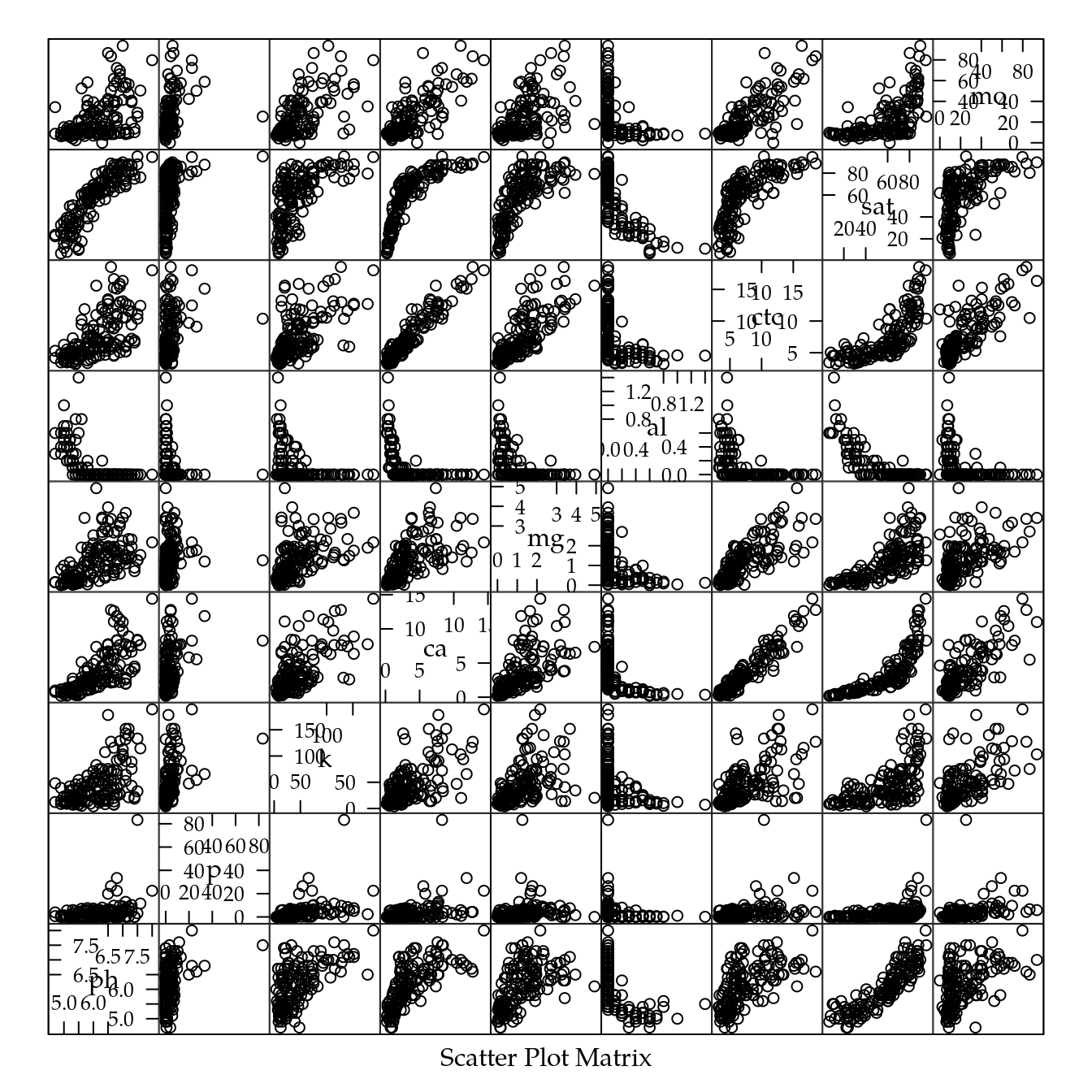

# Pares de diagramas de dispersão para as variáveis físicas.
splom(qui[, 11:15])

#-----------------------------------------------------------------------
# Agregando para a média das 3 camadas em cada local.

quim <- ddply(qui[, -2], .(loc), .fun = colMeans)
str(quim)

## 'data.frame':    50 obs. of  14 variables:
##  $ loc: num  1 2 3 4 5 6 7 8 9 10 ...
##  $ ph : num  6.73 4.77 7.1 5.93 5.63 ...
##  $ p  : num  7.78 1.56 4.53 9.27 1.43 ...
##  $ k  : num  31 23 55.7 26.3 30.9 ...
##  $ ca : num  4.503 0.647 4.357 2.847 1.647 ...
##  $ mg : num  1.327 0.1 1.31 0.713 0.893 ...
##  $ al : num  0 0.5 0 0.133 0.133 ...
##  $ ctc: num  7.85 4.31 7.91 5.95 5.01 ...
##  $ sat: num  72.1 17.6 72.1 53 45.8 ...
##  $ mo : num  35.8 17.6 25.2 22.8 19.9 ...
##  $ arg: num  228 227 218 190 330 ...
##  $ are: num  731 756 696 750 637 ...
##  $ cas: num  2.57 1.07 13.9 6.6 7.4 ...
##  $ acc: num  732 756 700 752 640 ...

splom(quim[, 2:10])

splom(quim[, 10:14])

Análise de Componentes Principais

Camadas como indivíduos

#-----------------------------------------------------------------------

# Cria uma matriz só com as variáveis de solo.
quiv <- qui[, -(1:2)]
rownames(quiv) <- with(qui, paste(loc, as.roman(as.numeric(cam)),
                                  sep = "-"))

acp <- princomp(quiv, cor = TRUE)

summary(acp)

## Importance of components:
##                           Comp.1    Comp.2     Comp.3     Comp.4
## Standard deviation     2.3854986 1.7376345 1.07551158 0.93098921
## Proportion of Variance 0.4377388 0.2322595 0.08897886 0.06667238
## Cumulative Proportion  0.4377388 0.6699983 0.75897712 0.82564950
##                            Comp.5     Comp.6     Comp.7     Comp.8
## Standard deviation     0.88988785 0.66322487 0.62727651 0.56409125
## Proportion of Variance 0.06091541 0.03383594 0.03026737 0.02447684
## Cumulative Proportion  0.88656491 0.92040085 0.95066823 0.97514507
##                            Comp.9     Comp.10     Comp.11
## Standard deviation     0.43024624 0.263392164 0.222279957
## Proportion of Variance 0.01423937 0.005336572 0.003800645
## Cumulative Proportion  0.98938444 0.994721010 0.998521655
##                             Comp.12      Comp.13
## Standard deviation     0.1056119374 0.0898031581
## Proportion of Variance 0.0008579909 0.0006203544
## Cumulative Proportion  0.9993796456 1.0000000000

# Proporção de variância acumulada.
plot(cbind(x = 0:length(acp$sdev),
           y = c(0, cumsum(acp$sdev^2))/sum(acp$sdev^2)),
     type = "o",
     xlab = "Componente",
     ylab = "Proporção de variância acumulada")
abline(h = 0.75, lty = 2)

#-----------------------------------------------------------------------
# Carregamentos.

# acp$loadings

# A fração dos carregamentos mais importantes.
imp <- function(x, f = 0.25) {
    a <- abs(x)
    k <- ceiling(f * length(x))
    i <- sort(a, decreasing = TRUE)[k]
    x[a <= i] <- NA
    return(x)
}

apply(acp$loadings[, 1:4], MARGIN = 2, FUN = imp, f = 0.25)

##        Comp.1     Comp.2     Comp.3     Comp.4
## ph         NA         NA         NA         NA
## p          NA         NA         NA  0.3540011
## k          NA         NA         NA         NA
## ca  0.3850495         NA         NA         NA
## mg         NA         NA         NA         NA
## al         NA         NA  0.1493058 -0.5714961
## ctc 0.3772880         NA         NA -0.3878400
## sat 0.3906511         NA         NA         NA
## mo         NA         NA         NA         NA
## arg        NA  0.5518568         NA         NA
## are        NA -0.5488643         NA         NA
## cas        NA         NA -0.8918405         NA
## acc        NA -0.5048946 -0.3669276         NA

#-----------------------------------------------------------------------
# Gráficos biplot.

biplot(acp, choices = c(1, 2))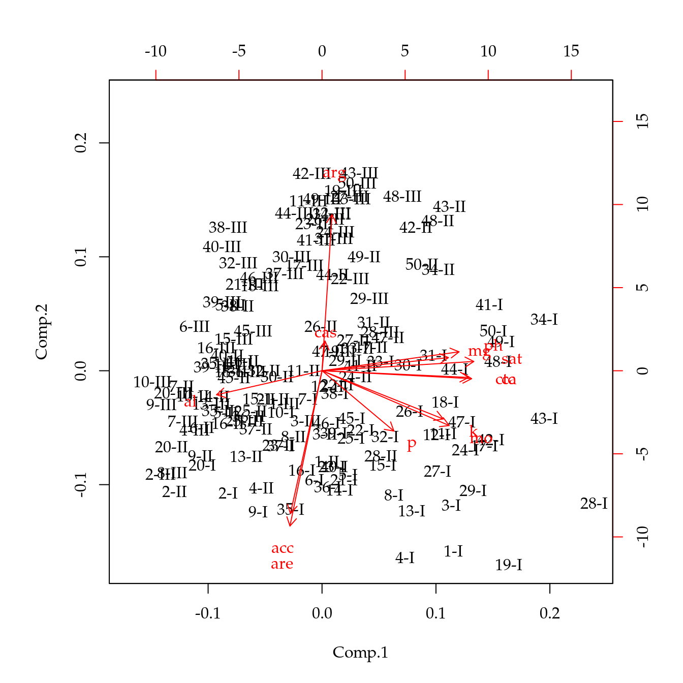

biplot(acp, choices = c(1, 3))

biplot(acp, choices = c(2, 3))

#-----------------------------------------------------------------------
# Indentifição das camadas.

# Escores.
sc <- acp$scores
pair <- c(1, 2)

# Aplitudes dos escores.
rgs <- apply(sc[, pair], MARGIN = 2, FUN = range)

# Carregamentos.
ld <- acp$loadings

# Amplitude dos carregamentos.
rgl <- apply(ld[, pair], MARGIN = 2, FUN = range)

# Fator de encolhimento para colocar setas em meio aos pontos.
f <- 0.5
xsc <- f * max(abs(rgs[, 1]))/max(abs(rgl[, 1]))
ysc <- f * max(abs(rgs[, 2]))/max(abs(rgl[, 2]))

par(pty = "s")
plot(rgs, col = "white", asp = 1,
     xlab = names(rgs)[1], ylab = names(rgs)[2])
points(sc[, pair], asp = 1, col = as.numeric(qui$cam), pch = 19)
abline(v = 0, h = 0, lty = 2)
arrows(x0 = rep(0, 1),
       y0 = rep(0, 1),
       x1 = ld[, pair[1]] * xsc,
       y1 = ld[, pair[2]] * ysc,
       length = 0.1,
       col = 2)
text(x = ld[, pair[1]] * xsc * 1.1,
     y = ld[, pair[2]] * ysc * 1.1,
     labels = rownames(ld))
legend("topleft", legend = levels(qui$cam),
       pch = 19, col = 1:3, bty = "n")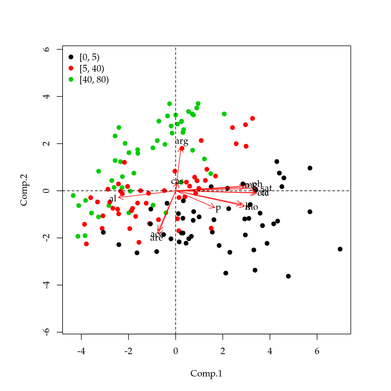

par(pty = "m")

Camadas como variáveis

#-----------------------------------------------------------------------

# Empilhar as variáveis de solo.
quie <- melt(data = qui,
             id.vars = c("loc", "cam"))
str(quie)

## 'data.frame':    1950 obs. of  4 variables:
##  $ loc     : int  1 1 1 2 2 2 3 3 3 4 ...
##  $ cam     : Factor w/ 3 levels "[0, 5)","[5, 40)",..: 1 2 3 1 2 3 1 2 3 1 ...
##  $ variable: Factor w/ 13 levels "ph","p","k","ca",..: 1 1 1 1 1 1 1 1 1 1 ...
##  $ value   : num  6.8 6.7 6.7 4.7 4.7 4.9 7.6 6.8 6.9 6.6 ...

quie$camvar <- with(quie, paste(as.character(variable),
                                as.character(as.roman(as.integer(cam))),
                                sep = ":"))

# Desempilhar as variáveis.
quie <- dcast(data = quie, formula = loc ~ camvar, value.var = "value")

str(quie)

## 'data.frame':    50 obs. of  40 variables:
##  $ loc    : int  1 2 3 4 5 6 7 8 9 10 ...
##  $ acc:I  : num  770 741 718 791 734 ...
##  $ acc:II : num  750 775 704 788 667 ...
##  $ acc:III: num  676 752 679 678 518 ...
##  $ al:I   : num  0 0.3 0 0 0 0 0 0 0 0.1 ...
##  $ al:II  : num  0 0.6 0 0 0.2 0.5 0.6 0 0.3 0.6 ...
##  $ al:III : num  0 0.6 0 0.4 0.2 0.6 0.8 0.7 1 1.4 ...
##  $ are:I  : num  770 741 716 790 733 ...
##  $ are:II : num  750 775 698 788 665 ...
##  $ are:III: num  674 752 674 674 514 ...
##  $ arg:I  : num  184 232 193 142 236 ...
##  $ arg:II : num  215 213 234 169 304 ...
##  $ arg:III: num  286 237 226 258 452 ...
##  $ ca:I   : num  8.27 0.97 7.63 5.54 2.99 1.88 1.6 5.82 1.91 1.73 ...
##  $ ca:II  : num  2.91 0.76 3.22 2.25 0.93 0.7 0.24 2.39 1.15 0.72 ...
##  $ ca:III : num  2.33 0.21 2.22 0.75 1.02 0.3 0.6 0.28 0.47 0.36 ...
##  $ cas:I  : num  1.8 0.4 8.4 5.5 5.5 20.9 12.4 2 1.4 0.8 ...
##  $ cas:II : num  2.2 1.1 19 3.1 7.2 23.4 2.9 2.1 2.5 1.6 ...
##  $ cas:III: num  3.7 1.7 14.3 11.2 9.5 31.8 5 3.6 3.3 1.4 ...
##  $ ctc:I  : num  12.47 5.3 12.41 9.11 7.57 ...
##  $ ctc:II : num  6.57 4.17 6.26 4.56 4.1 5.16 5.02 5.28 4.86 3.86 ...
##  $ ctc:III: num  4.52 3.47 5.06 4.18 3.37 4.48 4.53 3.61 4.58 4.54 ...
##  $ k:I    : num  72.2 48.1 114.5 54.3 56.8 ...
##  $ k:II   : num  13.4 12.3 25.8 11.1 22.2 ...
##  $ k:III  : num  7.23 8.64 26.83 13.57 13.57 ...
##  $ mg:I   : num  1.7 0.16 1.53 1.77 2.12 1.53 1.42 1.67 0.21 0.69 ...
##  $ mg:II  : num  1.77 0.14 1.31 0.21 0.52 0.36 0.14 0.99 0.05 0.37 ...
##  $ mg:III : num  0.51 0 1.09 0.16 0.04 0.1 0.18 0.28 0.04 0.12 ...
##  $ mo:I   : num  72.2 34.4 50.4 50.2 39.1 35 28.6 42.3 19.9 24.3 ...
##  $ mo:II  : num  25.6 8.7 15.6 10 11.2 5.8 8.5 11.8 6.3 6.9 ...
##  $ mo:III : num  9.7 9.7 9.5 8.2 9.3 9.3 8.2 7.6 7.1 8.8 ...
##  $ p:I    : num  22.51 3.89 11.52 26.43 3.79 ...
##  $ p:II   : num  0.83 0.69 1.66 1.17 0.49 0.69 0.21 1.14 1.36 1.04 ...
##  $ p:III  : num  0.01 0.1 0.41 0.2 0.01 0.1 0.01 0.01 1.07 0.1 ...
##  $ ph:I   : num  6.8 4.7 7.6 6.6 6 5.8 5.9 6.5 5.5 5.8 ...
##  $ ph:II  : num  6.7 4.7 6.8 6.2 5.1 5.2 5.1 6.4 4.9 5 ...
##  $ ph:III : num  6.7 4.9 6.9 5 5.8 5.5 5.6 5.1 5 5.5 ...
##  $ sat:I  : num  81.4 23.7 76.1 81.8 69.4 ...
##  $ sat:II : num  71.7 22.4 73.4 54.5 36.8 ...
##  $ sat:III: num  63.23 6.69 66.78 22.59 31.26 ...

#-----------------------------------------------------------------------

acp <- princomp(quie, cor = TRUE)

# summary(acp)

# Proporção de variância acumulada.
plot(cbind(x = 0:length(acp$sdev),
           y = c(0, cumsum(acp$sdev^2))/sum(acp$sdev^2)),
     type = "o",
     xlab = "Componente",
     ylab = "Proporção de variância acumulada")
abline(h = 0.75, lty = 2)

#-----------------------------------------------------------------------
# Carregamentos.

# acp$loadings

apply(acp$loadings[, 1:4], MARGIN = 2, FUN = imp, f = 0.25)

##            Comp.1     Comp.2     Comp.3     Comp.4
## loc            NA         NA  0.1908126         NA
## acc:I          NA -0.2238693         NA         NA
## acc:II         NA         NA  0.2270238 -0.1622790
## acc:III        NA         NA         NA -0.4100126
## al:I           NA         NA         NA         NA
## al:II          NA         NA         NA         NA
## al:III         NA         NA         NA         NA
## are:I          NA         NA         NA         NA
## are:II         NA -0.2585851         NA         NA
## are:III        NA         NA         NA -0.2484359
## arg:I          NA  0.2307062         NA         NA
## arg:II         NA  0.2516177         NA         NA
## arg:III        NA         NA         NA  0.3462011
## ca:I    0.2120379         NA         NA         NA
## ca:II   0.2024972         NA         NA         NA
## ca:III  0.2020180         NA         NA         NA
## cas:I          NA         NA  0.4528881         NA
## cas:II         NA         NA  0.4912041         NA
## cas:III        NA         NA  0.4324992 -0.1790642
## ctc:I   0.2128865         NA         NA         NA
## ctc:II  0.2094659         NA         NA         NA
## ctc:III        NA         NA  0.1545793         NA
## k:I            NA         NA         NA         NA
## k:II           NA -0.2500313  0.1710886         NA
## k:III          NA -0.2891170  0.1546419         NA
## mg:I           NA         NA -0.1973335         NA
## mg:II   0.1856483         NA         NA         NA
## mg:III         NA         NA         NA         NA
## mo:I           NA         NA         NA -0.1657718
## mo:II          NA         NA         NA         NA
## mo:III         NA         NA         NA         NA
## p:I            NA         NA         NA         NA
## p:II           NA -0.2969129         NA  0.3373342
## p:III          NA -0.2756235         NA  0.3858953
## ph:I           NA -0.2149295         NA         NA
## ph:II          NA         NA         NA -0.1686722
## ph:III         NA         NA         NA         NA
## sat:I   0.1924693         NA         NA         NA
## sat:II  0.2049075         NA         NA         NA
## sat:III 0.2144155         NA         NA         NA

#-----------------------------------------------------------------------
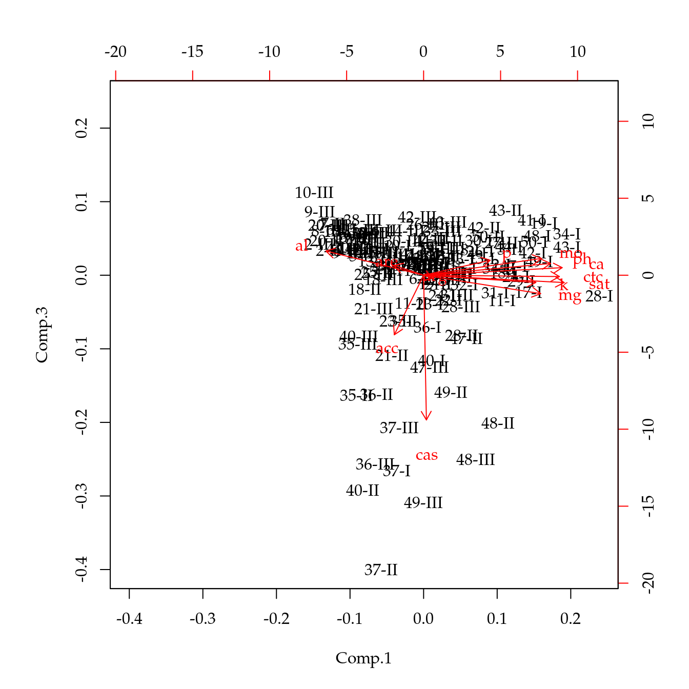
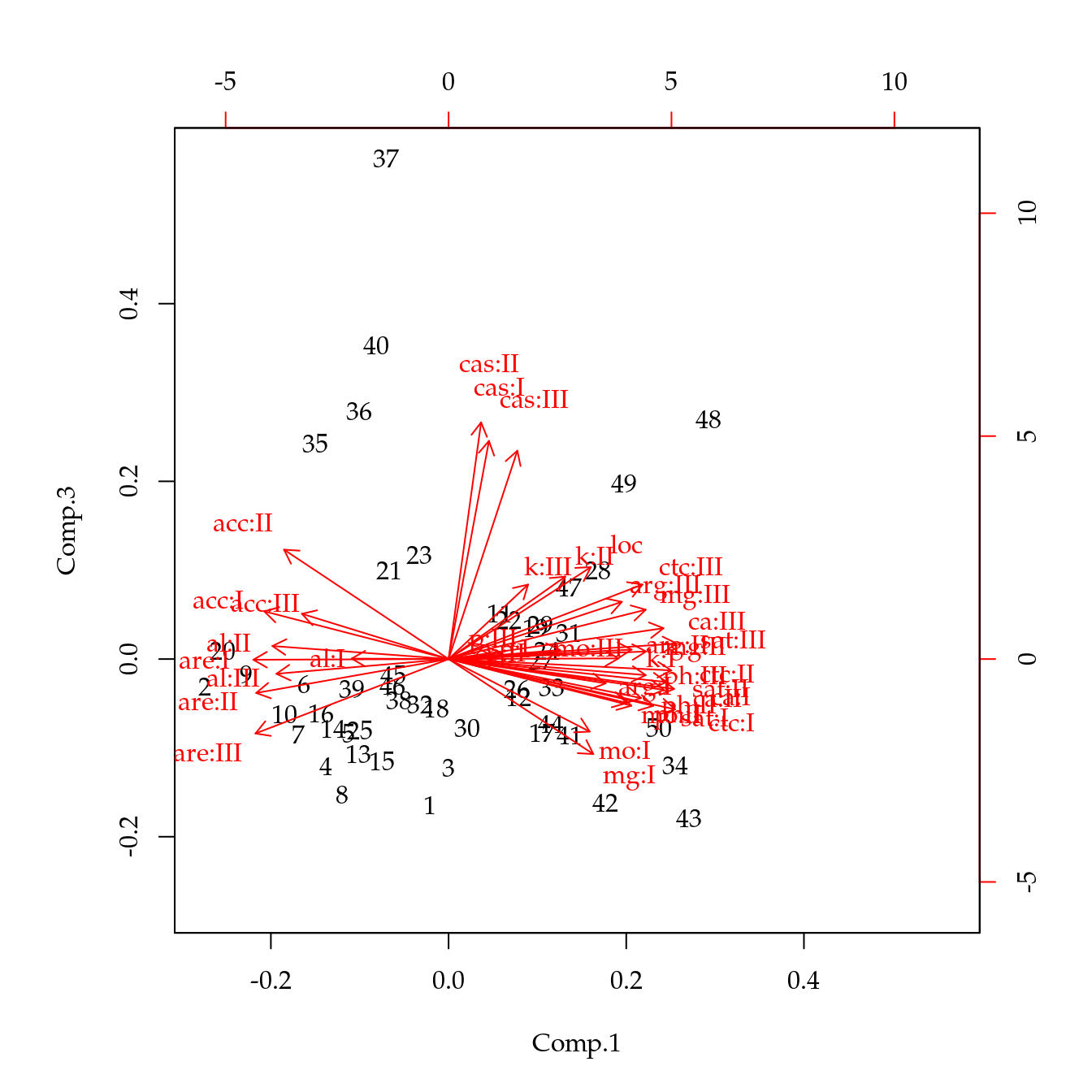
# Gráficos biplot.

biplot(acp, choices = c(1, 2))

biplot(acp, choices = c(1, 3))

biplot(acp, choices = c(2, 3))

Informações da Sessão

## Atualizado em 11 de julho de 2019.
## 
## R version 3.6.1 (2019-07-05)
## Platform: x86_64-pc-linux-gnu (64-bit)
## Running under: Ubuntu 18.04.2 LTS
## 
## Matrix products: default
## BLAS:   /usr/lib/x86_64-linux-gnu/blas/libblas.so.3.7.1
## LAPACK: /usr/lib/x86_64-linux-gnu/lapack/liblapack.so.3.7.1
## 
## locale:
##  [1] LC_CTYPE=pt_BR.UTF-8       LC_NUMERIC=C              
##  [3] LC_TIME=pt_BR.UTF-8        LC_COLLATE=en_US.UTF-8    
##  [5] LC_MONETARY=pt_BR.UTF-8    LC_MESSAGES=en_US.UTF-8   
##  [7] LC_PAPER=pt_BR.UTF-8       LC_NAME=C                 
##  [9] LC_ADDRESS=C               LC_TELEPHONE=C            
## [11] LC_MEASUREMENT=pt_BR.UTF-8 LC_IDENTIFICATION=C       
## 
## attached base packages:
## [1] stats     graphics  grDevices utils     datasets  methods  
## [7] base     
## 
## other attached packages:
## [1] reshape2_1.4.3      plyr_1.8.4          EACS_0.0-7         
## [4] wzRfun_0.91         captioner_2.2.3     latticeExtra_0.6-28
## [7] RColorBrewer_1.1-2  lattice_0.20-38     knitr_1.23         
## 
## loaded via a namespace (and not attached):
##  [1] Rcpp_1.0.1        compiler_3.6.1    prettyunits_1.0.2
##  [4] remotes_2.1.0     tools_3.6.1       testthat_2.1.1   
##  [7] digest_0.6.20     pkgbuild_1.0.3    pkgload_1.0.2    
## [10] evaluate_0.14     memoise_1.1.0     rlang_0.4.0      
## [13] rstudioapi_0.10   cli_1.1.0         commonmark_1.7   
## [16] yaml_2.2.0        pkgdown_1.3.0     xfun_0.8         
## [19] withr_2.1.2       stringr_1.4.0     roxygen2_6.1.1   
## [22] xml2_1.2.0        desc_1.2.0        fs_1.3.1         
## [25] devtools_2.1.0    rprojroot_1.3-2   grid_3.6.1       
## [28] glue_1.3.1        R6_2.4.0          processx_3.4.0   
## [31] rmarkdown_1.13    sessioninfo_1.1.1 callr_3.3.0      
## [34] magrittr_1.5      usethis_1.5.1     backports_1.1.4  
## [37] ps_1.3.0          htmltools_0.3.6   MASS_7.3-51.4    
## [40] assertthat_0.2.1  stringi_1.4.3     crayon_1.3.4

Análise Exploratória

Análise de Componentes Principais

Camadas como indivíduos

Camadas como variáveis

Informações da Sessão

Contents