|
|
Linguagens de Programação para Ciência de DadosExploração e comunicação de dados com R e Python |
Visualização de Dados com ggplot2
Walmes Zeviani
Introdução
Este tutorial é orientado à perguntas. Para cada pergunta, portanto, tem-se a manipulação e visualização de dados correspondente. São dadas explicações para o que não é considerado autoexplicativo no código.
Definições da sessão
# Carrega o conjunto de pacotes do tidyverse.
library(tidyverse)

library(esquisse)     # Shiny para construir gráficos com drag & drop.
library(DataExplorer) # Recursos ágeis de visualização.
Imóveis à venda em Curitiba
Os dados de imóveis foram coletados pelos alunos Hektor Brasil e Alcides Neto que os utilizaram em seu trabalho de conclusão de curso.
Importação e preparação dos dados
#-----------------------------------------------------------------------
# Importar arquivos com dados sobre imóveis a venda em Curitiba.

# Endereço dos dados.
url <- "http://leg.ufpr.br/~walmes/data/TCC_Brasil_Neto/ImoveisWeb-Realty.csv"

# Cria diretório para manter dados se não existir.
if (!dir.exists("./data")) {
    dir.create(path = "./data")
}

# Baixa arquivo para diretório caso não exista.
path <- "./data/ImoveisWeb-Realty.csv"
if (!file.exists(path)) {
    download.file(url, destfile = path)
}

# Importa o arquivo para o ambiente.
imo <- read_csv2(path, locale = locale(encoding = "latin1"))
## Using ',' as decimal and '.' as grouping mark. Use read_delim() for more control.## Parsed with column specification:
## cols(
## .default = col_double(),
## url = col_character(),
## type = col_character(),
## title = col_character(),
## description = col_character(),
## address = col_character(),
## advertiser = col_character(),
## CRECI = col_character()
## )## See spec(...) for full column specifications.attr(imo, "spec") <- NULL
# Estrutura do arquivo de dados.
str(imo, vec.len = 3, nchar.max = 30)## Classes 'spec_tbl_df', 'tbl_df', 'tbl' and 'data.frame': 71316 obs. of 22 variables:
## $ id : num 1 2 3 4 5 6 7 8 ...
## $ url : chr "propriedades/"| __truncated__ "propriedades/"| __truncated__ "propriedades/"| __truncated__ ...
## $ type : chr "Apartamento" "Casa" "Apartamento" ...
## $ title : chr "excelente opo"| __truncated__ "Residencial M"| __truncated__ "Apartamento r"| __truncated__ ...
## $ description: chr "\nDescrição O"| __truncated__ "\nResidencial"| __truncated__ "\nEmpreendime"| __truncated__ ...
## $ address : chr "Avenida Iguaç"| __truncated__ "Rua Barão de "| __truncated__ "Rua Antônio G"| __truncated__ ...
## $ lat : num -25.4 -25.5 -25.5 -25.4 ...
## $ lon : num -49.3 -49.2 -49.3 -49.3 ...
## $ pictures : num 31 8 31 3 10 50 6 3 ...
## $ iptu : num 720 NA NA NA NA NA NA NA ...
## $ condominium: num 430 NA NA NA NA 1100 NA 100 ...
## $ usefulArea : num 75 107 56 500 NA 266 131 49 ...
## $ totalArea : num 95 107 99 500 769 429 131 76 ...
## $ bedroom : num 2 3 2 NA NA 3 NA NA ...
## $ suite : num 1 1 1 NA NA 3 NA NA ...
## $ bathroom : num 2 1 2 NA NA 6 1 1 ...
## $ garage : num 2 1 1 NA NA 5 NA NA ...
## $ price : num 649900 460000 395000 490000 ...
## $ years : num 5 NA NA NA NA 3 NA NA ...
## $ publishment: num 2 31 108 13 347 99 192 NA ...
## $ advertiser : chr "PRIME SOHO IMÓVEIS P33" "HABITARTE IMÓVEIS" "M.A Corretora de Imoveis" ...
## $ CRECI : chr NA "3929J" "F22018" ...# Contagem do tipo de imóvel.
imo %>%
count(type)## # A tibble: 5 x 2
## type n
## <chr> <int>
## 1 Apartamento 47200
## 2 Casa 15001
## 3 Comercial 4308
## 4 Rural 61
## 5 Terreno 4746# Aplicação de filtros.
imo <- imo %>%
filter(is.element(type, c("Casa", "Apartamento")),
bedroom <= 20,
between(price, left = 10^4, right = 10^7),
between(usefulArea, left = 1.1 * 10^1, right = 3 * 10^3),
between(lon, left = -49.40, right = -49.15),
between(lat, left = -25.65, right = -25.30)) %>%
select(lat,
lon,
type,
pictures,
bedroom,
suite,
bathroom,
garage,
usefulArea,
iptu,
condominium,
price)
# Dados de apartamentos para trabalhar.
str(imo)## Classes 'spec_tbl_df', 'tbl_df', 'tbl' and 'data.frame': 48713 obs. of 12 variables:
## $ lat : num -25.4 -25.5 -25.5 -25.4 -25.4 ...
## $ lon : num -49.3 -49.2 -49.3 -49.3 -49.3 ...
## $ type : chr "Apartamento" "Casa" "Apartamento" "Apartamento" ...
## $ pictures : num 31 8 31 50 12 14 21 25 35 26 ...
## $ bedroom : num 2 3 2 3 4 2 4 2 3 3 ...
## $ suite : num 1 1 1 3 4 1 1 2 1 1 ...
## $ bathroom : num 2 1 2 6 NA 2 3 3 1 4 ...
## $ garage : num 2 1 1 5 4 1 2 2 1 3 ...
## $ usefulArea : num 75 107 56 266 339 89 168 120 138 149 ...
## $ iptu : num 720 NA NA NA NA NA 201 NA 102 NA ...
## $ condominium: num 430 NA NA 1100 NA NA 890 NA 990 NA ...
## $ price : num 649900 460000 395000 2100000 4525100 ...Conhecendo a estrutura dos dados
O pacote DataExplorer tem recursos para um rápido exame dos dados que consiste de conhecer a tipagem das variáveis, proporção de missing, etc.
# Tabela de frequência por tipo de variável.
introduce(imo) %>% t()
## [,1]
## rows 48713
## columns 12
## discrete_columns 1
## continuous_columns 11
## all_missing_columns 0
## total_missing_values 82393
## complete_rows 7159
## total_observations 584556
## memory_usage 4679904# Versão gráfica da tipagem e condição das variáveis.
plot_intro(imo)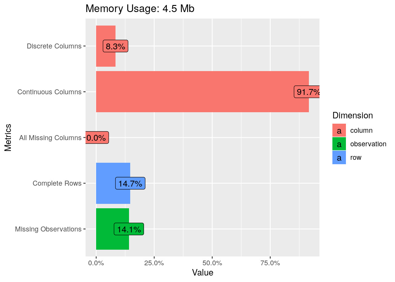
# Gráfico de proporção de missing por variável.
plot_missing(imo)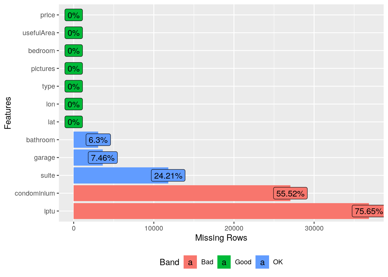
Distribuição de frequência
# Gráfico de barras para as variáveis qualitativas.
plot_bar(imo)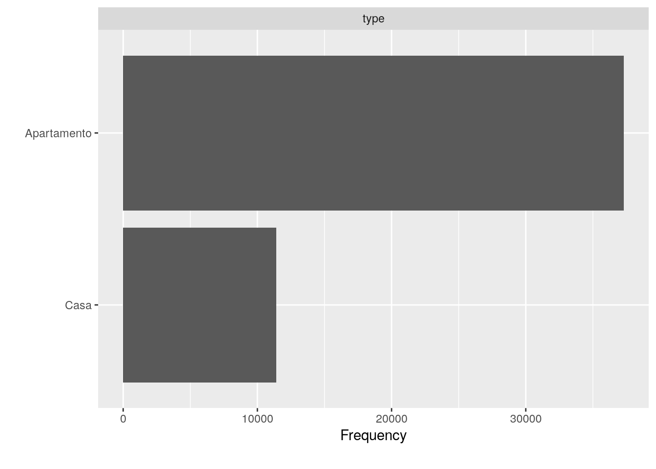
# Historgama para as variáveis quantitativas.
plot_histogram(imo)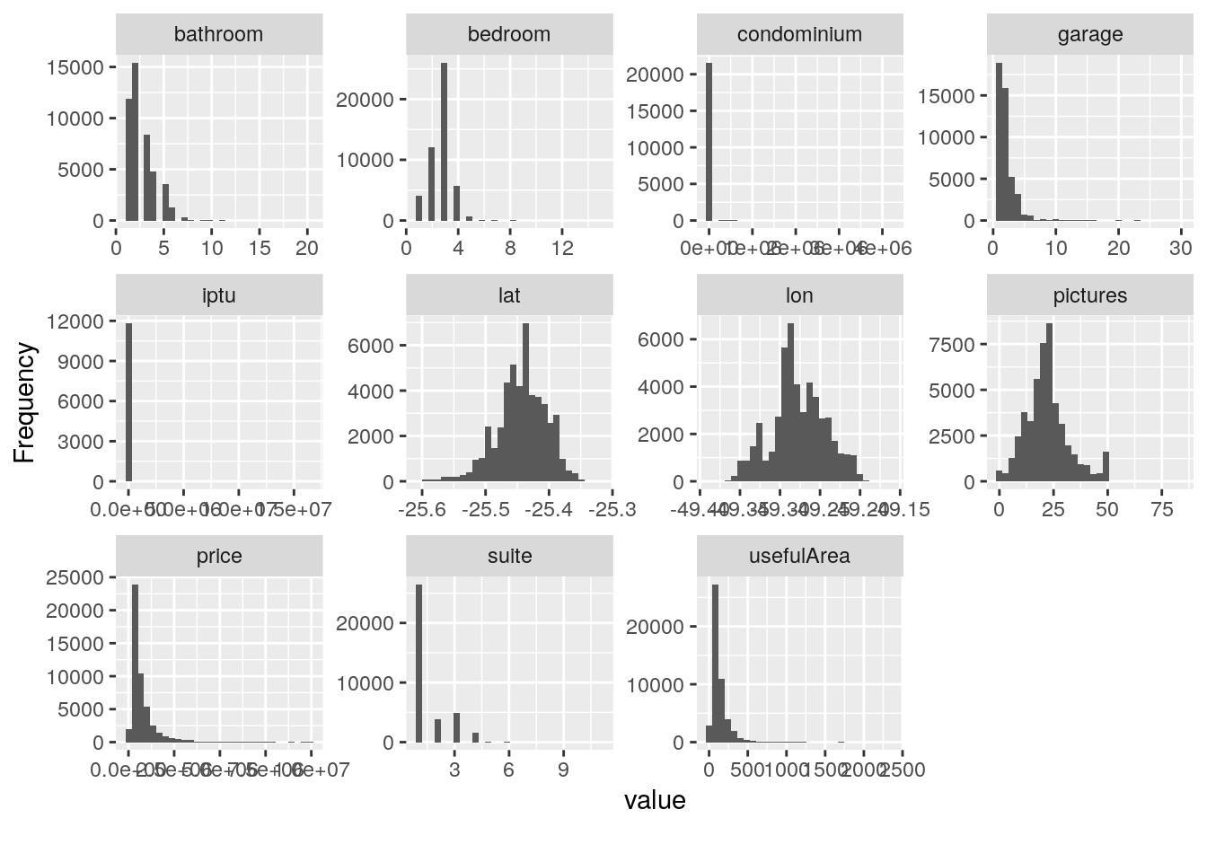
Gráficos orientados à perguntas
# Qual a distribuição do tamanho por tipo de imóvel?
ggplot(data = imo, mapping = aes(x = usefulArea)) +
    facet_wrap(facets = ~type, ncol = 1) +
    geom_histogram(fill = "cyan4", color = "black") +
    scale_x_log10()
## `stat_bin()` using `bins = 30`. Pick better value with `binwidth`.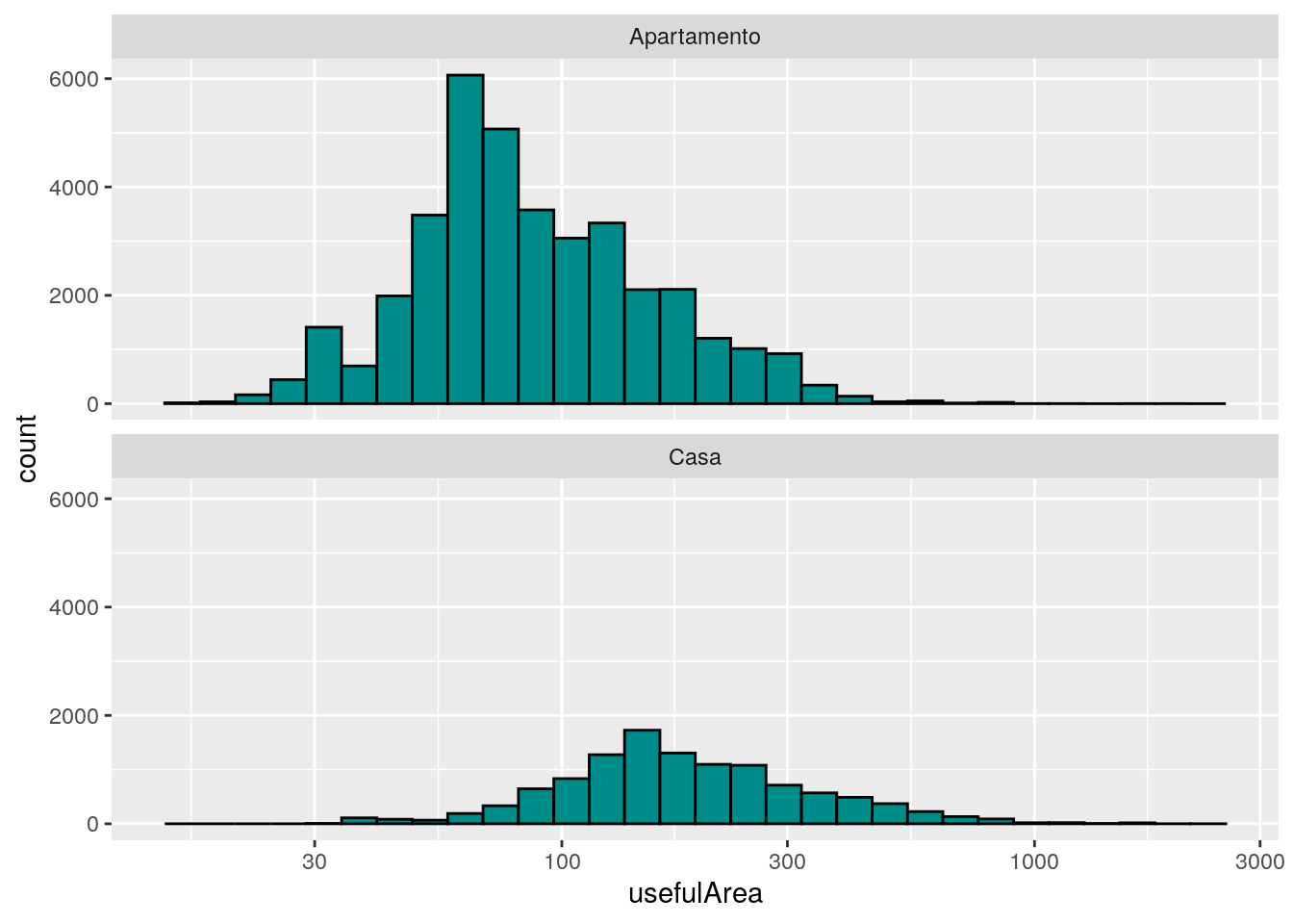
ggplot(data = imo, mapping = aes(x = usefulArea, fill = type)) +
    geom_density(color = "black", alpha = 0.25) +
    scale_x_log10()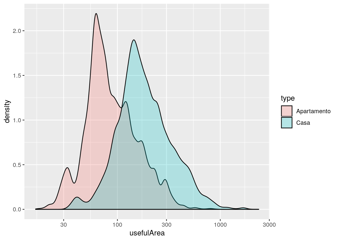
# Qual a distribuição do preço por tipo de imóvel?
ggplot(data = imo, mapping = aes(x = price)) +
    facet_wrap(facets = ~type, ncol = 1) +
    geom_histogram(fill = "cyan4", color = "black") +
    scale_x_log10()
## `stat_bin()` using `bins = 30`. Pick better value with `binwidth`.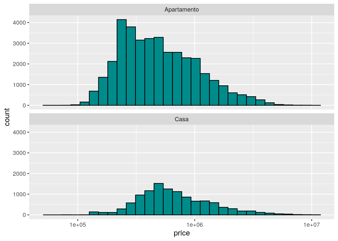
ggplot(data = imo, mapping = aes(x = price, fill = type)) +
    geom_density(color = "black", alpha = 0.25) +
    scale_x_log10()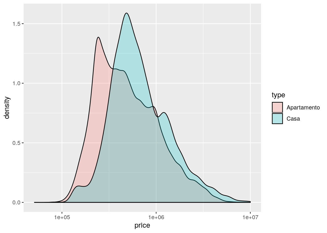
# Como combinar o histograma com a densidade?
ggplot(data = imo, mapping = aes(x = price)) +
    geom_histogram(aes(y = ..density.., fill = ..density..)) +
    geom_density() +
    geom_rug() +
    scale_x_log10() +
    labs(x = "Preço de venda",
         y = "Frequência absoluta")
## `stat_bin()` using `bins = 30`. Pick better value with `binwidth`.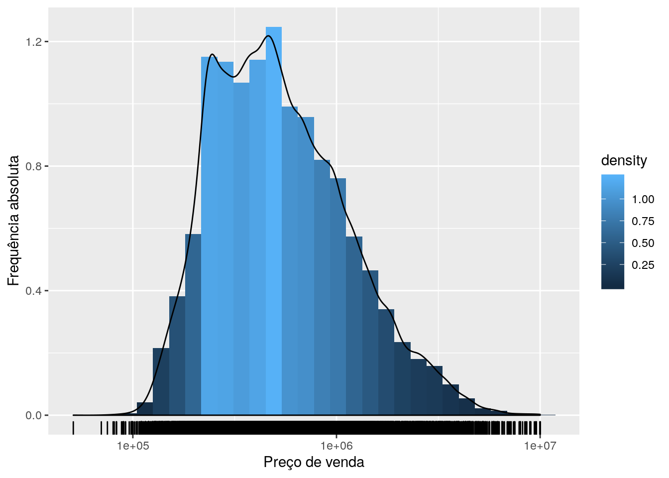
# Qual a distribuição número de quartos por tipo de imóvel?
ggplot(data = imo, mapping = aes(x = bedroom)) +
    facet_wrap(facets = ~type, ncol = 1) +
    geom_histogram(fill = "cyan4", color = "black", binwidth = 1)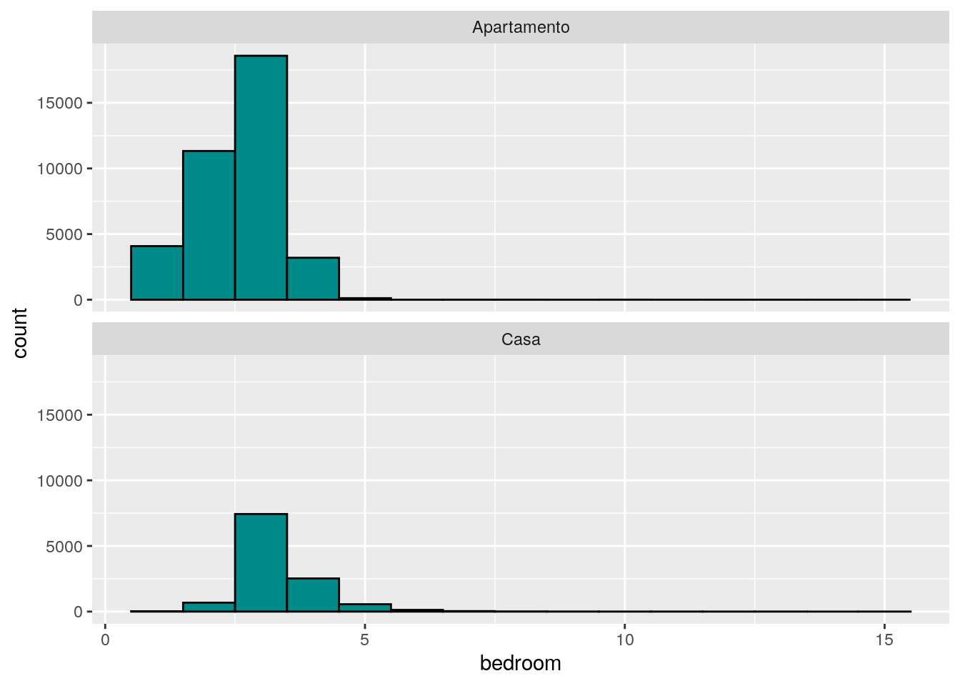
# Qual a distribuição do valor do condomínio?
ggplot(data = filter(imo, condominium < 10000),
       mapping = aes(x = condominium, fill = type)) +
    geom_density(color = "black", alpha = 0.25)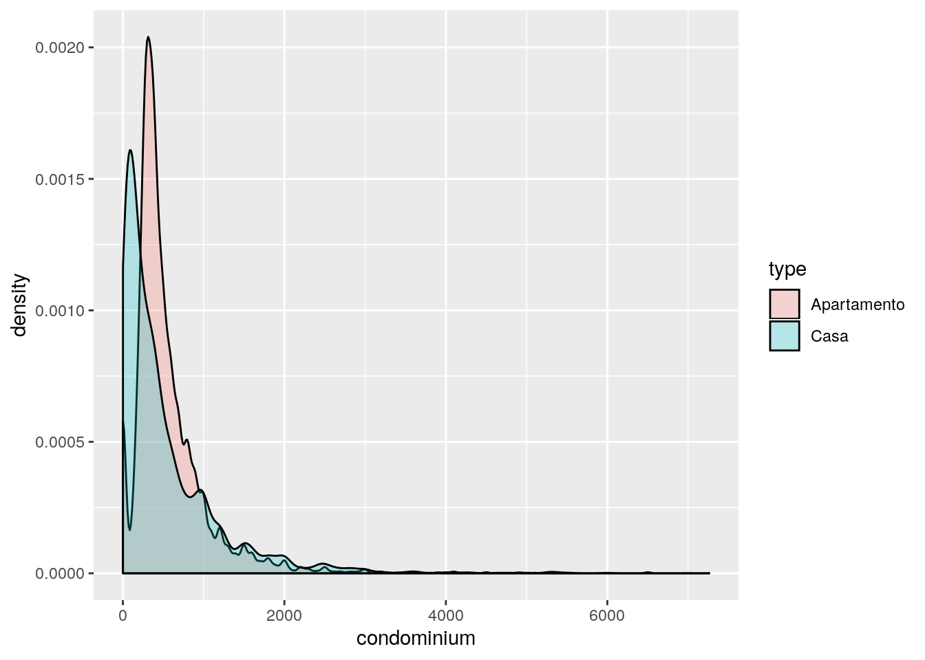
# O valor ausente no condomínio depende o valor de venda?
ggplot(data = imo,
       mapping = aes(x = price, color = is.na(condominium))) +
    facet_wrap(facets = ~type) +
    geom_step(stat = "ecdf") +
    scale_x_log10()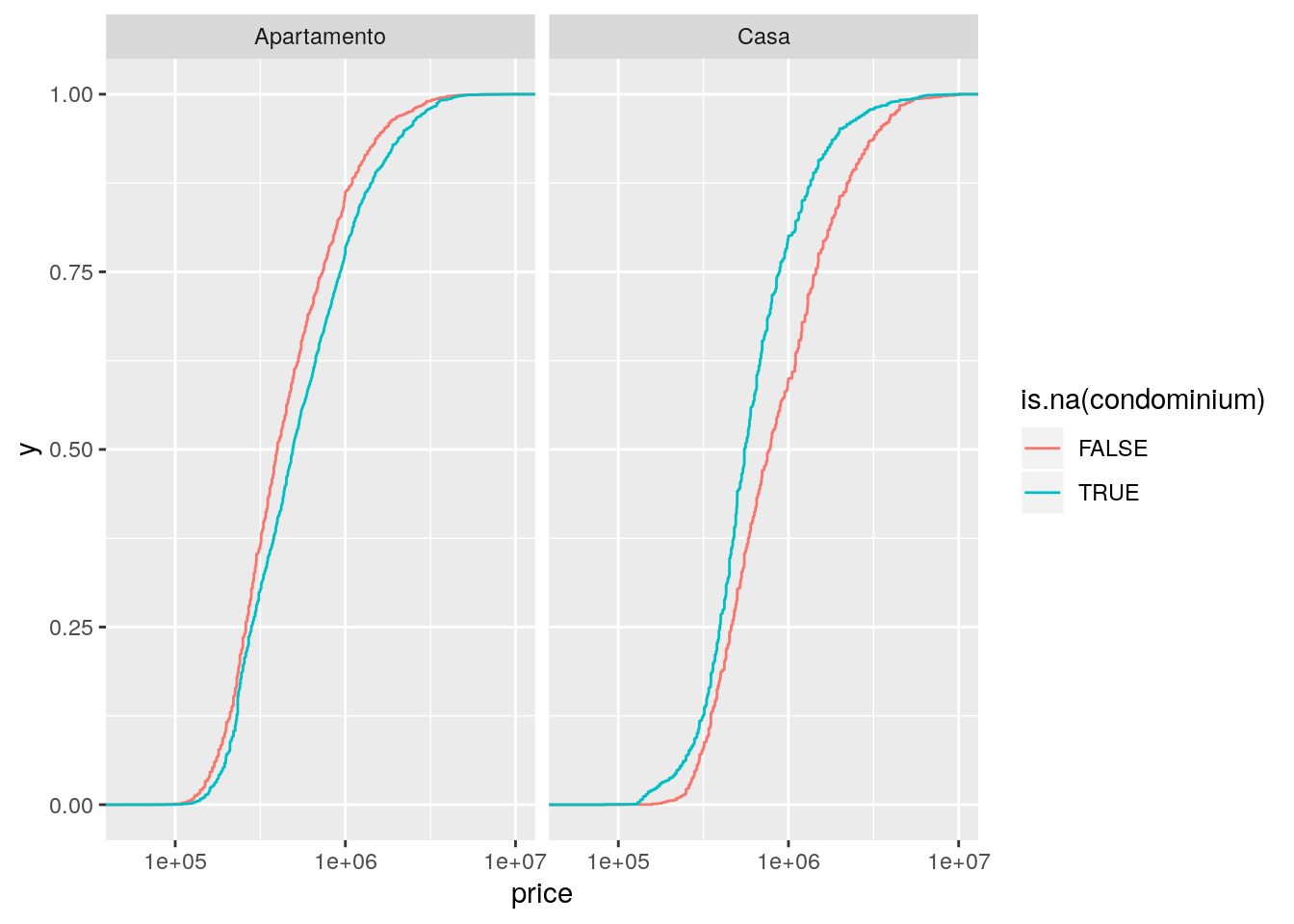
# O valor do ausente no IPTU depende o valor de venda?
ggplot(data = imo,
       mapping = aes(x = price, color = is.na(iptu))) +
    facet_wrap(facets = ~type) +
    geom_step(stat = "ecdf") +
    scale_x_log10()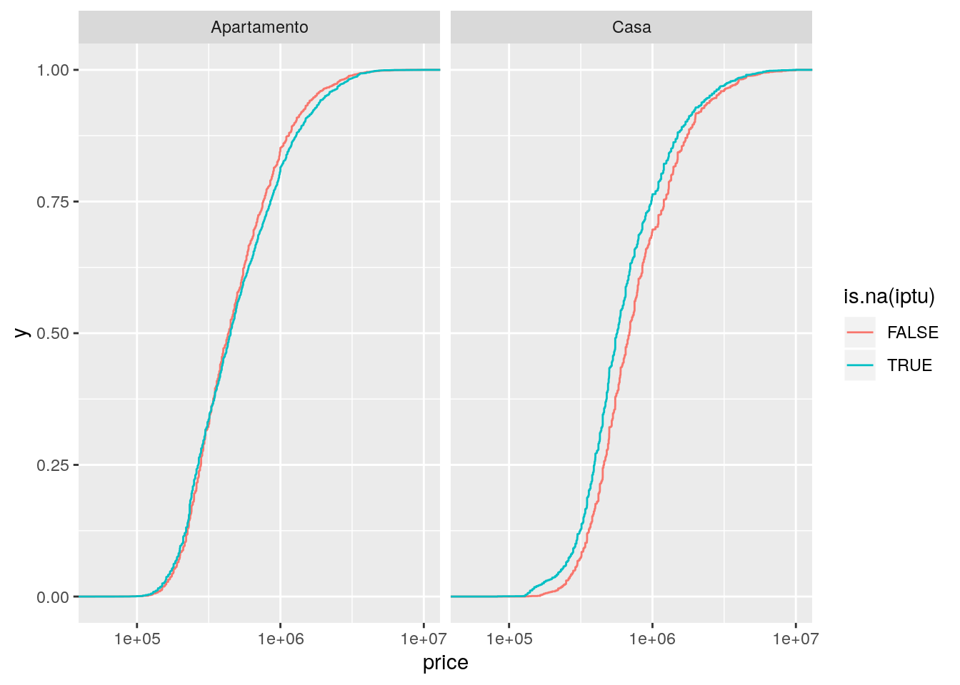
# Qual a distribuição conjunta dos missings em IPTU e condomínio?
ggplot(data = imo,
       mapping = aes(x = is.na(condominium), fill = is.na(iptu))) +
    facet_wrap(facets = ~type) +
    geom_bar()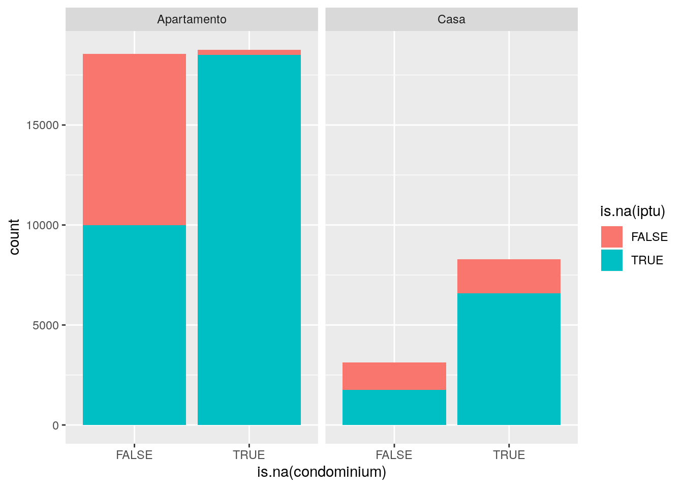
ggplot(data = imo,
       mapping = aes(x = is.na(condominium), fill = is.na(iptu))) +
    facet_wrap(facets = ~type) +
    geom_bar(position = "fill")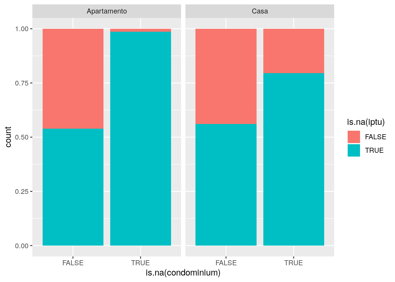
ggplot(data = imo,
       mapping = aes(x = is.na(condominium), fill = is.na(iptu))) +
    facet_wrap(facets = ~type) +
    geom_bar(position = "dodge")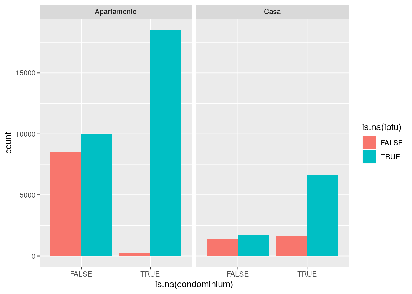
# Qual a relação entre preço e área?
ggplot(data = imo,
       mapping = aes(x = usefulArea, y = price)) +
    facet_wrap(facets = ~type) +
    geom_point()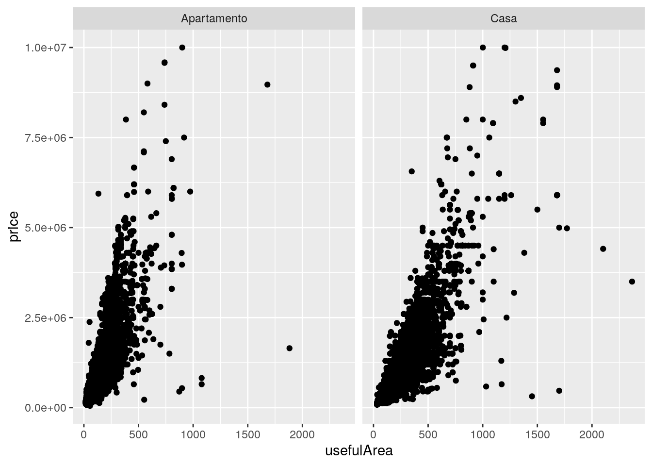
ggplot(data = imo,
       mapping = aes(x = usefulArea, y = price)) +
    facet_wrap(facets = ~type) +
    geom_point(pch = 1, alpha = 0.5) +
    geom_smooth(se = FALSE, color = "darkorange") +
    scale_x_log10() +
    scale_y_log10()
## `geom_smooth()` using method = 'gam' and formula 'y ~ s(x, bs = "cs")'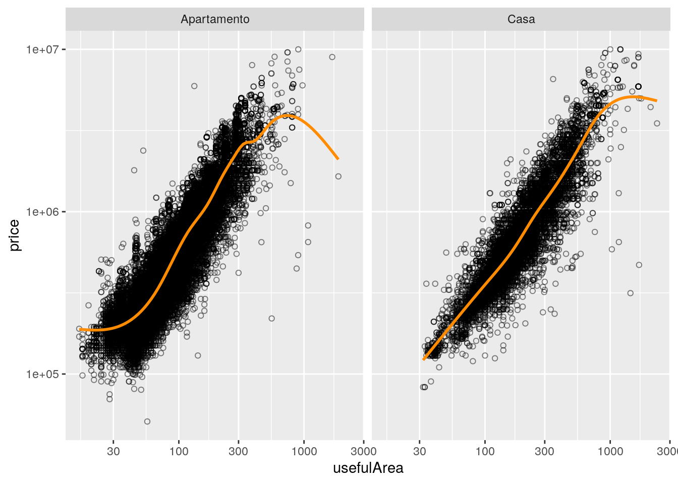
ggplot(data = imo,
       mapping = aes(x = usefulArea, y = price, color = type)) +
    geom_point(pch = 1, alpha = 0.5) +
    geom_smooth(se = FALSE, show.legend = TRUE) +
    scale_x_log10() +
    scale_y_log10()
## `geom_smooth()` using method = 'gam' and formula 'y ~ s(x, bs = "cs")'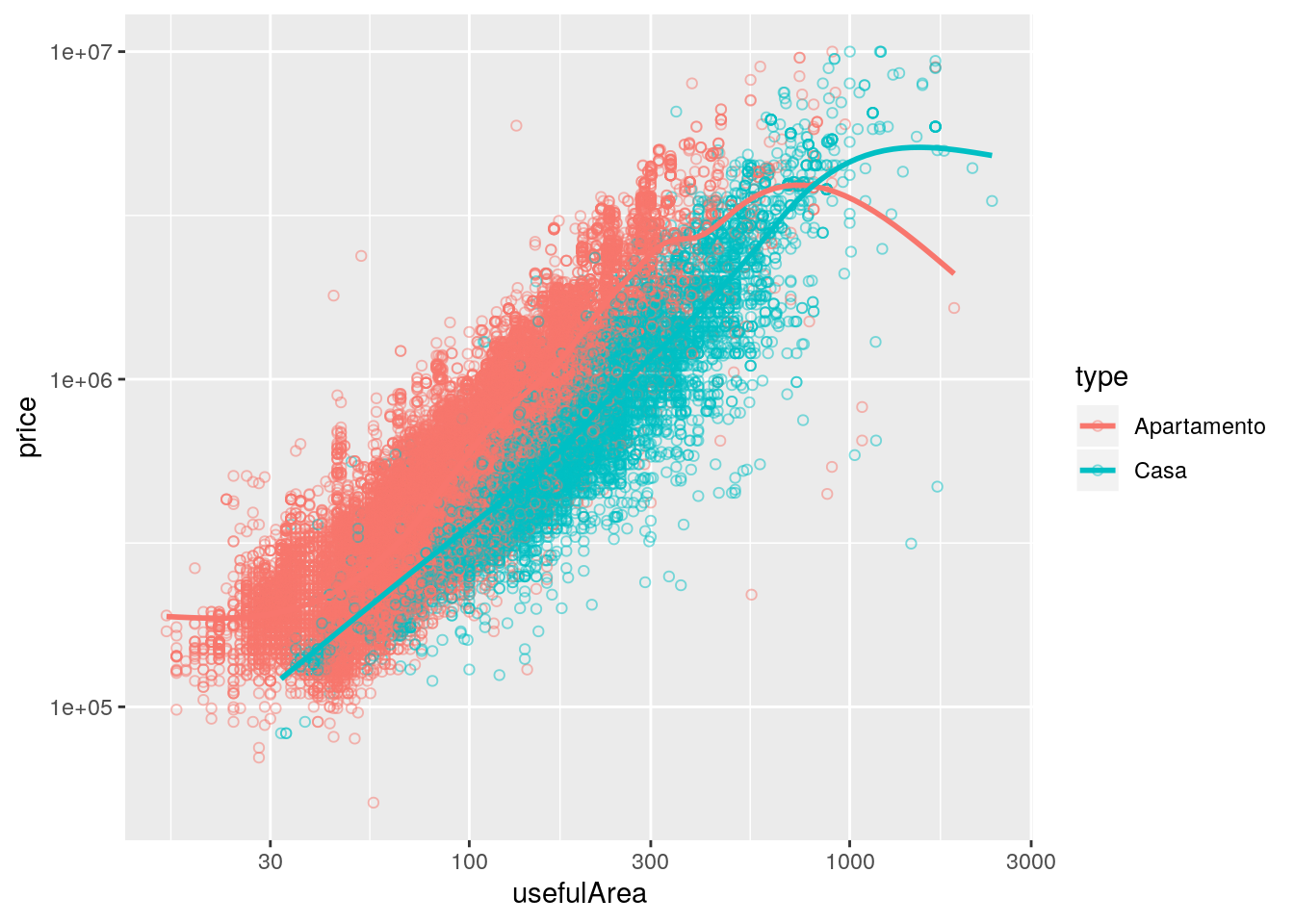
Dados de HB-20 à venda
# Importação.
url <- "http://leg.ufpr.br/~walmes/data/hb20_venda_webmotors_280314.txt"
hb <- read_tsv(url)

# Remove o atributo "spec".
attr(hb, "spec") <- NULL

# Estrutura do objeto.
str(hb)

hb %>%
    count(carro)

ggplot(hb, aes(x = km,
               y = preco,
               color = carro,
               group = carro)) +
    geom_point() +
    geom_smooth(method = "lm")

tb <- hb %>%
    filter(carro == "hb20")

tb

ggplot(hb, aes(x = km,
               y = preco,
               color = carro,
               group = carro)) +
    geom_point() +
    geom_smooth(method = "lm")

mean(tb[tb$km == 0, ]$preco)

coef(lm(preco ~ km + I(km^2), data = tb[tb$km > 0, ]))

ggplot(hb, aes(x = km,
               y = preco,
               color = anomod)) +
    geom_point() +
    geom_smooth(method = "lm",
                aes(group = 1)) +
    facet_wrap(facet = ~carro)

ggplot(hb, aes(x = km,
               y = preco,
               color = anomod)) +
    geom_point() +
    geom_smooth(method = "lm",
                aes(group = 1)) +
    facet_grid(facet = anomod ~ carro)
Dados de jogadores do Brasileirão 2018
# Pode usar 2016, 2017 ou 2018.
url <- "http://leg.ufpr.br/~walmes/data/jogadores-brasileirao-2018.txt"
bra8 <- read_tsv(url)

# Remove o atributo "spec".
attr(bra8, "spec") <- NULL

# Estrutura do objeto.
str(bra8)

bra8$Height[bra8$Height < 150] <- NA
bra8$Weight[bra8$Weight < 30] <- NA

ggplot(bra8, aes(x = Height)) +
    geom_density()

ggplot(bra8, aes(x = Weight)) +
    geom_density()

ggplot(bra8, aes(x = Height, y = Weight)) +
    # geom_point()
    geom_jitter()

ggplot(bra8, aes(x = Height, y = Weight)) +
    # geom_point() +
    # geom_density2d() +
    # geom_hex()
    geom_bin2d()

ggplot(bra8,
       aes(x = Height,
           y = Weight,
           size = Age)) +
    geom_point(pch = 1) +
    # geom_smooth(guide = FALSE) +
    facet_wrap(facets = ~PositionText)
Usando a interface do Esquisse
library(esquisse)

esquisser(imo)

esquisser(bra8)

esquisser(hb)|
Linguagens de Programação para Ciência de Dados leg.ufpr.br/~walmes/ensino/dsbd-linprog |
Prof. Walmes M. Zeviani Departamento de Estatística · UFPR |