Links úteis:

#-----------------------------------------------------------------------
# Pacotes.

# Para fazer ensaios de performance.
library(microbenchmark)
ls("package:microbenchmark")
# help(microbenchmark, h = "html")

# Troca as opções default da função.
formals(microbenchmark)$times <- 10

# Carrega pacote, exibe versão e funções/objetos públicos.
library(data.table)
packageVersion("data.table")
ls("package:data.table")

library(tidyverse)

1 Leitura de arquivo

Serão usados vários conjuntos de dados nesse tutorial comparativo. O primeiro deles TODO

#-----------------------------------------------------------------------
# Carregando um conjunto de dados do repositório de ML.

# browseURL("http://archive.ics.uci.edu/ml/datasets/Bank+Marketing")

# URL do arquivo.
u <- "http://archive.ics.uci.edu/ml/machine-learning-databases/00222/bank.zip"

if (!file.exists(basename(u))) {
    download.file(u, destfile = basename(u))
    utils::unzip(zipfile = basename(u))
}

# Coleção de arquivos.
dir(pattern = "^bank")

## [1] "bank-full.csv"  "bank-names.txt" "bank.csv"       "bank.zip"

system("wc -l bank-full.csv")     # Conta o número de linhas.
system("head -n 3 bank-full.csv") # Mostra o topo do arquivo.
system("file -bi bank-full.csv")  # Exibe o mimetype e encoding.

1.1 R básico

# Carregando o arquivo com utils::read.csv2().
da_bs <- read.csv2(file = "bank-full.csv",
                   stringsAsFactors = FALSE)
str(da_bs)

## 'data.frame':    45211 obs. of  17 variables:
##  $ age      : int  58 44 33 47 33 35 28 42 58 43 ...
##  $ job      : chr  "management" "technician" "entrepreneur" "blue-collar" ...
##  $ marital  : chr  "married" "single" "married" "married" ...
##  $ education: chr  "tertiary" "secondary" "secondary" "unknown" ...
##  $ default  : chr  "no" "no" "no" "no" ...
##  $ balance  : int  2143 29 2 1506 1 231 447 2 121 593 ...
##  $ housing  : chr  "yes" "yes" "yes" "yes" ...
##  $ loan     : chr  "no" "no" "yes" "no" ...
##  $ contact  : chr  "unknown" "unknown" "unknown" "unknown" ...
##  $ day      : int  5 5 5 5 5 5 5 5 5 5 ...
##  $ month    : chr  "may" "may" "may" "may" ...
##  $ duration : int  261 151 76 92 198 139 217 380 50 55 ...
##  $ campaign : int  1 1 1 1 1 1 1 1 1 1 ...
##  $ pdays    : int  -1 -1 -1 -1 -1 -1 -1 -1 -1 -1 ...
##  $ previous : int  0 0 0 0 0 0 0 0 0 0 ...
##  $ poutcome : chr  "unknown" "unknown" "unknown" "unknown" ...
##  $ y        : chr  "no" "no" "no" "no" ...

1.2 DT

# Lendo com a data.table::fread().
da_dt <- fread(file = "bank-full.csv",
               header = TRUE,
               sep = ";")
str(da_dt)

## Classes 'data.table' and 'data.frame':   45211 obs. of  17 variables:
##  $ age      : int  58 44 33 47 33 35 28 42 58 43 ...
##  $ job      : chr  "management" "technician" "entrepreneur" "blue-collar" ...
##  $ marital  : chr  "married" "single" "married" "married" ...
##  $ education: chr  "tertiary" "secondary" "secondary" "unknown" ...
##  $ default  : chr  "no" "no" "no" "no" ...
##  $ balance  : int  2143 29 2 1506 1 231 447 2 121 593 ...
##  $ housing  : chr  "yes" "yes" "yes" "yes" ...
##  $ loan     : chr  "no" "no" "yes" "no" ...
##  $ contact  : chr  "unknown" "unknown" "unknown" "unknown" ...
##  $ day      : int  5 5 5 5 5 5 5 5 5 5 ...
##  $ month    : chr  "may" "may" "may" "may" ...
##  $ duration : int  261 151 76 92 198 139 217 380 50 55 ...
##  $ campaign : int  1 1 1 1 1 1 1 1 1 1 ...
##  $ pdays    : int  -1 -1 -1 -1 -1 -1 -1 -1 -1 -1 ...
##  $ previous : int  0 0 0 0 0 0 0 0 0 0 ...
##  $ poutcome : chr  "unknown" "unknown" "unknown" "unknown" ...
##  $ y        : chr  "no" "no" "no" "no" ...
##  - attr(*, ".internal.selfref")=<externalptr>

1.3 TV

# Lendo com a readr::read_csv().
da_tv <- read_csv2(file = "bank-full.csv")

## Using ',' as decimal and '.' as grouping mark. Use read_delim() for more control.

## Parsed with column specification:
## cols(
##   age = col_integer(),
##   job = col_character(),
##   marital = col_character(),
##   education = col_character(),
##   default = col_character(),
##   balance = col_integer(),
##   housing = col_character(),
##   loan = col_character(),
##   contact = col_character(),
##   day = col_integer(),
##   month = col_character(),
##   duration = col_integer(),
##   campaign = col_integer(),
##   pdays = col_integer(),
##   previous = col_integer(),
##   poutcome = col_character(),
##   y = col_character()
## )

str(da_tv, give.attr = FALSE)

## Classes 'tbl_df', 'tbl' and 'data.frame':    45211 obs. of  17 variables:
##  $ age      : int  58 44 33 47 33 35 28 42 58 43 ...
##  $ job      : chr  "management" "technician" "entrepreneur" "blue-collar" ...
##  $ marital  : chr  "married" "single" "married" "married" ...
##  $ education: chr  "tertiary" "secondary" "secondary" "unknown" ...
##  $ default  : chr  "no" "no" "no" "no" ...
##  $ balance  : int  2143 29 2 1506 1 231 447 2 121 593 ...
##  $ housing  : chr  "yes" "yes" "yes" "yes" ...
##  $ loan     : chr  "no" "no" "yes" "no" ...
##  $ contact  : chr  "unknown" "unknown" "unknown" "unknown" ...
##  $ day      : int  5 5 5 5 5 5 5 5 5 5 ...
##  $ month    : chr  "may" "may" "may" "may" ...
##  $ duration : int  261 151 76 92 198 139 217 380 50 55 ...
##  $ campaign : int  1 1 1 1 1 1 1 1 1 1 ...
##  $ pdays    : int  -1 -1 -1 -1 -1 -1 -1 -1 -1 -1 ...
##  $ previous : int  0 0 0 0 0 0 0 0 0 0 ...
##  $ poutcome : chr  "unknown" "unknown" "unknown" "unknown" ...
##  $ y        : chr  "no" "no" "no" "no" ...

1.4 benchmark

res <- microbenchmark(
    "R básico" = {
        read.csv2(file = "bank-full.csv",
                  stringsAsFactors = FALSE)
    },
    "DT" = {
        fread(file = "bank-full.csv",
              header = TRUE,
              sep = ";")
    },
    "TV" = {
        suppressMessages(read_csv2(file = "bank-full.csv"))
    },
    times = 25)
res

## Unit: milliseconds
##      expr       min        lq      mean    median        uq       max
##  R básico 127.29657 131.85065 138.54201 132.92953 138.00520 200.29525
##        DT  16.72783  17.57623  20.91354  18.22800  19.78224  78.23218
##        TV  57.99802  59.00746  61.52231  59.27475  61.84736  96.87909
##  neval cld
##     25   c
##     25 a  
##     25  b

boxplot(res)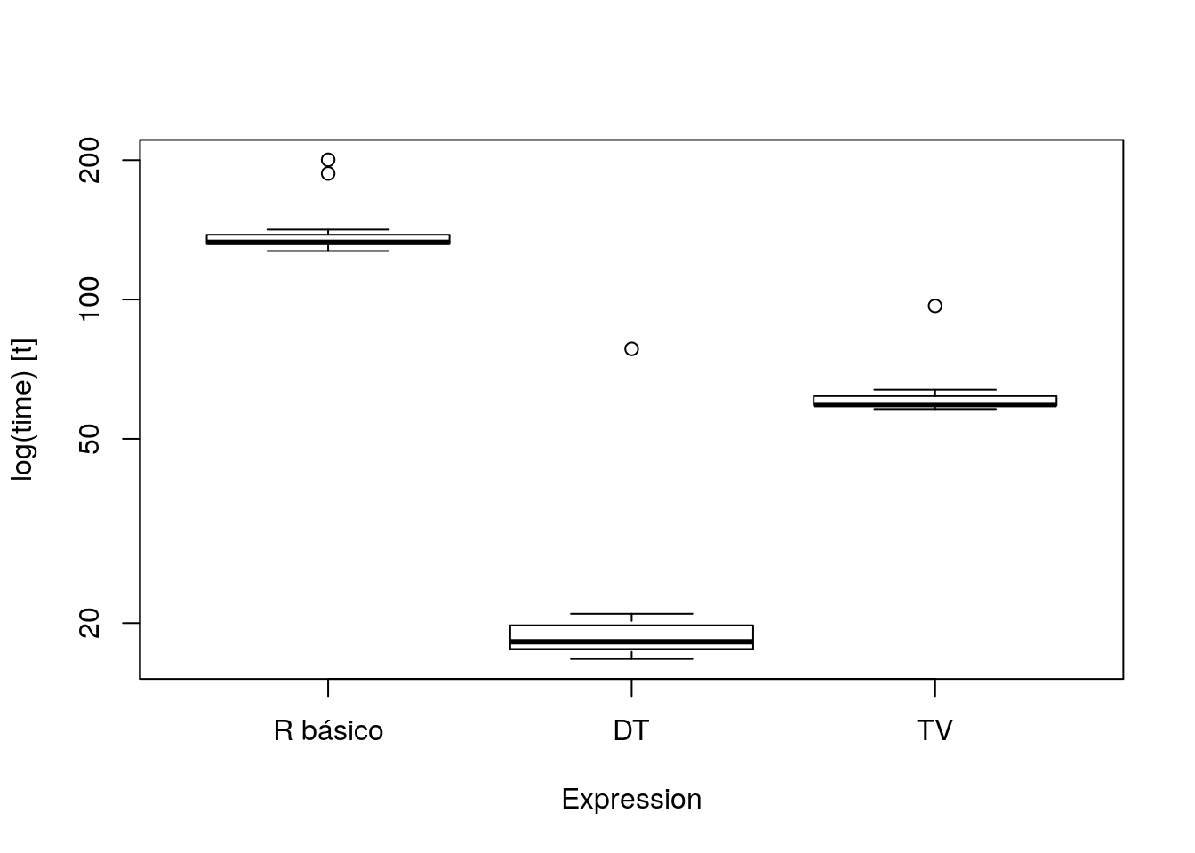

2 Ordenar as linhas

2.1 R básico

da_bs <- da_bs[order(da_bs$age), ]
da_bs <- da_bs[order(da_bs$marital, da_bs$age, decreasing = TRUE), ]
rbind(head(da_bs), tail(da_bs))

##       age         job  marital education default balance housing loan
## 42461  86     retired   single secondary      no     614      no   no
## 31052  83     retired   single   primary      no    3349      no   no
## 41790  83     retired   single   primary      no    1965      no   no
## 41523  77     retired   single   primary      no     300      no   no
## 41424  73     retired   single secondary      no    1050      no   no
## 43214  73     retired   single secondary      no    1050      no   no
## 6935   25 blue-collar divorced secondary      no    2428     yes   no
## 8960   25 blue-collar divorced secondary      no     720     yes   no
## 13287  25  technician divorced secondary      no      86      no  yes
## 35585  25  technician divorced  tertiary      no    2317     yes   no
## 40518  25    services divorced secondary      no    1694      no   no
## 38567  24 blue-collar divorced secondary      no     513     yes   no
##         contact day month duration campaign pdays previous poutcome   y
## 42461 telephone   9   dec      595        1    -1        0  unknown yes
## 31052 telephone  12   feb       89        1    -1        0  unknown  no
## 41790 telephone  13   oct     1003        3    -1        0  unknown yes
## 41523  cellular   9   sep      511        1    -1        0  unknown  no
## 41424  cellular   4   sep       73        2    -1        0  unknown  no
## 43214  cellular   4   mar      562        3   181        2  failure yes
## 6935    unknown  28   may      376        4    -1        0  unknown  no
## 8960    unknown   4   jun      156        1    -1        0  unknown  no
## 13287  cellular   8   jul      483        2    -1        0  unknown  no
## 35585  cellular   7   may      273        4    -1        0  unknown  no
## 40518  cellular   7   jul      159        2    -1        0  unknown  no
## 38567  cellular  15   may       61        3    -1        0  unknown  no

2.2 DT

da_dt <- da_dt[order(age)]
da_dt <- da_dt[order(marital, age, decreasing = TRUE)]

setorder(da_dt, marital, -age)
setorderv(da_dt, cols = c("marital", "age"), order = c(1, -1))
da_dt

##        age     job  marital education default balance housing loan
##     1:  95 retired divorced   primary      no    2282      no   no
##     2:  94 retired divorced secondary      no    1234      no   no
##     3:  90 retired divorced secondary      no       1      no   no
##     4:  90 retired divorced   primary      no     712      no   no
##     5:  89 retired divorced   primary      no    1323      no   no
##    ---                                                            
## 45207:  18 student   single secondary      no     156      no   no
## 45208:  18 student   single   primary      no     608      no   no
## 45209:  18 student   single   unknown      no     108      no   no
## 45210:  18 student   single   unknown      no     348      no   no
## 45211:  18 student   single   unknown      no     438      no   no
##          contact day month duration campaign pdays previous poutcome   y
##     1: telephone  21   apr      207       17    -1        0  unknown yes
##     2:  cellular   3   mar      212        1    -1        0  unknown  no
##     3:  cellular  13   feb      152        3    -1        0  unknown yes
##     4: telephone   3   mar      557        1    -1        0  unknown yes
##     5: telephone  29   dec      207        4   189        1    other  no
##    ---                                                                  
## 45207:  cellular   4   nov      298        2    82        4    other  no
## 45208:  cellular  13   nov      210        1    93        1  success yes
## 45209:  cellular   9   feb       92        1   183        1  success yes
## 45210:  cellular   5   may      443        4    -1        0  unknown yes
## 45211:  cellular   1   sep      425        1    -1        0  unknown  no

2.3 TV

da_tv <- arrange(da_tv, age)
da_tv <- arrange(da_tv, marital, -age)
da_tv

## # A tibble: 45,211 x 17
##      age job     marital  education default balance housing loan  contact 
##    <int> <chr>   <chr>    <chr>     <chr>     <int> <chr>   <chr> <chr>   
##  1    95 retired divorced primary   no         2282 no      no    telepho…
##  2    94 retired divorced secondary no         1234 no      no    cellular
##  3    90 retired divorced secondary no            1 no      no    cellular
##  4    90 retired divorced primary   no          712 no      no    telepho…
##  5    89 retired divorced primary   no         1323 no      no    telepho…
##  6    87 retired divorced primary   no         6746 no      no    telepho…
##  7    86 retired divorced primary   no            0 no      no    telepho…
##  8    86 retired divorced unknown   no          157 no      no    telepho…
##  9    85 retired divorced primary   no         7613 no      no    cellular
## 10    84 retired divorced primary   no         2619 no      no    telepho…
## # ... with 45,201 more rows, and 8 more variables: day <int>, month <chr>,
## #   duration <int>, campaign <int>, pdays <int>, previous <int>,
## #   poutcome <chr>, y <chr>

2.4 benchmark

res <- microbenchmark(
    "R básico" = {
        x <- da_bs[order(da_bs$marital,
                         sample(c(-1, 1), size = 1) * da_bs$age), ]
    },
    "DT" = {
        setorderv(da_dt,
                  cols = c("marital", "age"),
                  order = c(1, sample(c(-1, 1), size = 1)))
    },
    "TV" = {
        x <- arrange(da_tv,
                     marital,
                     sample(c(-1, 1), size = 1) * age)
    },
    times = 50)
res

## Unit: microseconds
##      expr       min        lq      mean    median        uq       max
##  R básico 18740.169 19336.129 21443.427 19944.630 21357.106  68534.31
##        DT   419.249   537.033  4200.173  1603.168  1712.223 108441.08
##        TV 11961.889 12208.998 16141.571 16595.196 16876.948  63634.56
##  neval cld
##     50   c
##     50 a  
##     50  b

boxplot(res)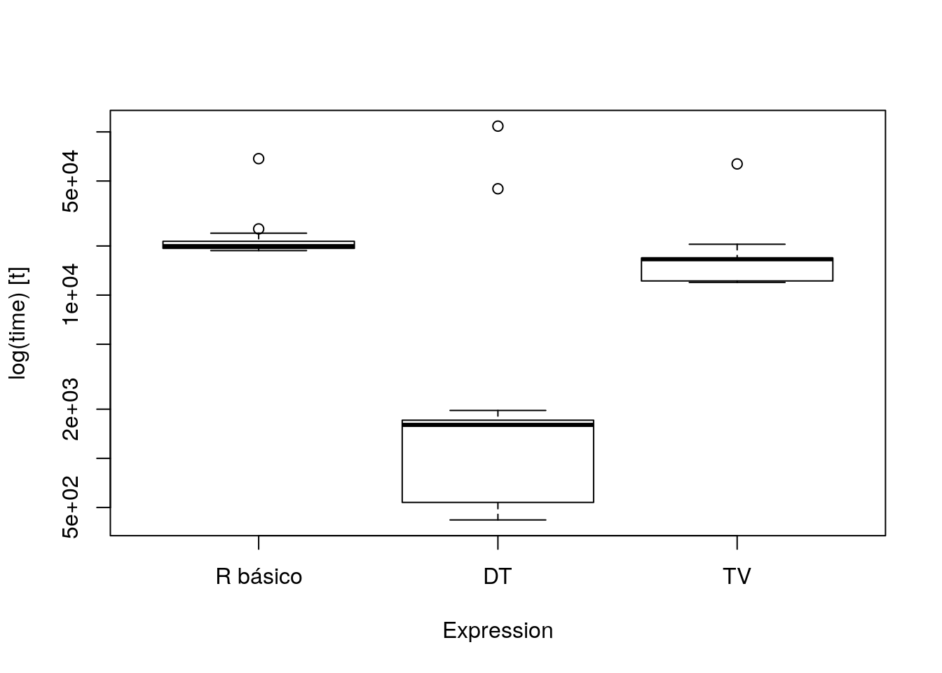

3 Filtros nas linhas

3.1 R básico

tb <- da_bs[da_bs$age > 70, ]
tb <- da_bs[da_bs$age > 50 & da_bs$marital == "divorced", ]
tb <- da_bs[da_bs$balance >= 1000 & da_bs$balance <= 2000, ]

tb <- subset(da_bs, age > 70)
tb <- subset(da_bs, age > 50 & marital == "divorced")
tb <- subset(da_bs, balance >= 1000 & balance <= 2000)

3.2 DT

tb <- da_dt[age > 70]
tb <- da_dt[age > 50 & marital == "divorced"]
tb <- da_dt[balance >= 1000 & balance <= 2000]
tb <- da_dt[data.table::between(balance, lower = 1000, upper = 2000)]

tb <- subset(da_bs, age > 70)
tb <- subset(da_bs, age > 50 & marital == "divorced")
tb <- subset(da_bs, balance >= 1000 & balance <= 2000)
tb <- subset(da_bs, data.table::between(balance, lower = 1000, upper = 2000))

3.3 TV

tb <- filter(da_tv, age > 70)
tb <- filter(da_tv, age > 50, marital == "divorced")
tb <- filter(da_tv, balance >= 1000 & balance <= 2000)
tb <- filter(da_tv, dplyr::between(balance, left = 1000, right = 2000))

3.4 benchmark

u <- unique(da_bs$marital) # Valores para estado civil.
x <- range(da_bs$age)      # Domínio dos valores de idade.

res <- microbenchmark(
    "R básico []" = {
        xi <- floor(runif(n = 1, min(x), max(x)))
        ui <- sample(u, size = 1)
        da <- da_bs[da_bs$age > xi & da_bs$marital == ui, ]
    },
    "DT []" = {
        xi <- floor(runif(n = 1, min(x), max(x)))
        ui <- sample(u, size = 1)
        da <- da_dt[age > xi & marital == ui]
    },
    "R básico subset"= {
        xi <- floor(runif(n = 1, min(x), max(x)))
        ui <- sample(u, size = 1)
        da <- subset(da_bs, age > xi & marital == ui)
    },
    "DT subset" = {
        xi <- floor(runif(n = 1, min(x), max(x)))
        ui <- sample(u, size = 1)
        da <- subset(da_dt, age > xi & marital == ui)
    },
    "TV" = {
        xi <- floor(runif(n = 1, min(x), max(x)))
        ui <- sample(u, size = 1)
        da <- filter(da_tv, age > xi, marital == ui)
    },
    times = 200)
res

## Unit: microseconds
##             expr      min        lq      mean    median        uq      max
##      R básico []  867.407  948.7695 1755.0968 1102.1950 1857.6385 7928.080
##            DT []  519.287  620.6015  900.6334  696.4730  870.8555 4965.807
##  R básico subset 1008.106 1109.2585 1779.5182 1263.5435 1711.1780 7905.186
##        DT subset  613.918  743.6395 1077.7073  844.5385 1148.7220 5389.892
##               TV  586.189  713.5805 1130.0608  813.7325 1152.3700 6238.018
##  neval cld
##    200   b
##    200  a 
##    200   b
##    200  a 
##    200  a

boxplot(res)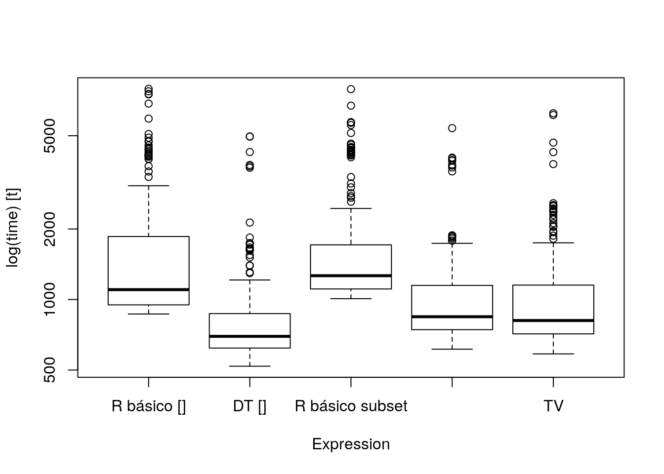

4 Seleção de variáveis

4.1 R básico

tb <- da_bs[, c("age", "marital", "education")]
tb <- da_dt[, c(1:4, 7, 10:12)]
tb <- da_dt[, -c(1:4, 7, 10:12)]
tb <- Filter(f = is.numeric, x = da_bs)

tb <- subset(da_bs, select = c("age", "marital", "education"))
tb <- subset(da_bs, select = c(age, marital, education))
tb <- subset(da_bs, select = -c(age, marital, education))
tb <- subset(da_bs, select = c(1:4, 7, 10:12))
tb <- subset(da_bs, select = -c(1:4, 7, 10:12))

4.2 DT

tb <- da_dt[, c("age", "marital", "education")]
tb <- da_dt[, -c("age", "marital", "education")]
tb <- da_dt[, !c("age", "marital", "education")]
tb <- da_dt[, list(age, marital, education)]
tb <- da_dt[, c(1:4, 7, 10:12)]
tb <- da_dt[, -c(1:4, 7, 10:12)]
tb <- Filter(f = is.numeric, x = da_dt)
tb <- da_dt[, Filter(f = is.numeric, x = .SD)]

tb <- subset(da_dt, select = c("age", "marital", "education"))
tb <- subset(da_dt, select = c(age, marital, education))
tb <- subset(da_dt, select = -c(age, marital, education))
tb <- subset(da_dt, select = c(1:4, 7, 10:12))
tb <- subset(da_dt, select = -c(1:4, 7, 10:12))

4.3 TV

tb <- select(da_tv, age, marital, education)
tb <- select(da_tv, -age, -marital, -education)
tb <- select(da_tv, c(age, marital, education))
tb <- select(da_tv, -c(age, marital, education))
tb <- select(da_tv, c("age", "marital", "education"))
tb <- select(da_tv, c(1:4, 7, 10:12))
tb <- select(da_tv, -c(1:4, 7, 10:12))
tb <- select(da_tv, -c(1:4, 7, 10:12))
tb <- select_if(da_tv, .predicate = is.numeric)

4.4 benchmark

v <- names(da_bs)

res <- microbenchmark(
    "R básico []"     = da_bs[, sample(v, size = 5)],
    "DT []"           = da_dt[, sample(v, size = 5)],
    "R básico subset" = subset(da_bs, select = sample(v, size = 5)),
    "DT subset"       = subset(da_dt, select = sample(v, size = 5)),
    "TV"              = select(da_dt, sample(v, size = 5)),
    times = 300)
res

## Unit: microseconds
##             expr      min        lq       mean    median        uq
##      R básico []   14.824   28.3195   34.15823   36.2360   39.9105
##            DT []  139.851  176.5995  587.97342  209.4805  256.4375
##  R básico subset 5432.716 5711.3340 6110.54962 5811.6255 5941.7750
##        DT subset  418.908  526.1330  640.25265  576.0300  635.9735
##               TV  768.419  845.0265  972.11030 1007.1550 1064.1220
##         max neval cld
##     135.972   300 a  
##  110897.137   300 ab 
##   12299.640   300   c
##    4077.956   300 ab 
##    2644.261   300  b

boxplot(res)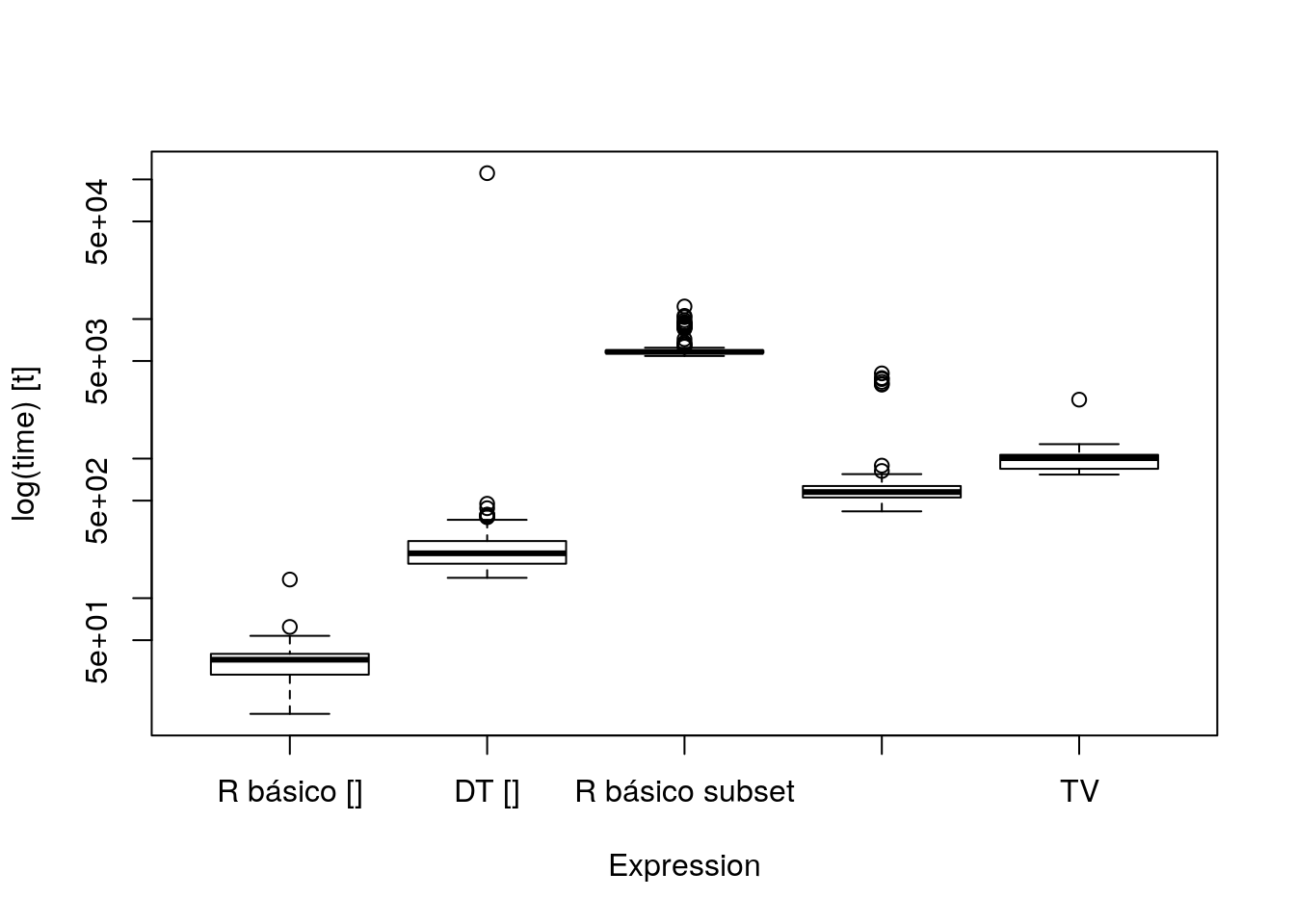

5 Transformação de variáveis

5.1 R básico

tb <- da_bs[, 1:17]
tb$x <- log(tb$age)
tb$y <- tb$education %in% c("tertiary", "secondary")
str(tb)

tb <- da_bs[, 1:17]
tb <- transform(tb,
                x = log(age),
                y = education %in% c("tertiary", "secondary"))
str(tb)

tb <- da_bs[, 1:17]
tb <- within(tb, {
    x <- log(age)
    y <- education %in% c("tertiary", "secondary")
})
str(tb)

5.2 DT

tb <- da_dt[, 1:17]
tb$x <- log(tb$age)
tb$y <- tb$education %in% c("tertiary", "secondary")
str(tb)

tb <- da_dt[, 1:17]
tb <- transform(tb,
                x = log(age),
                y = education %in% c("tertiary", "secondary"))
str(tb)

tb <- da_dt[, 1:17]
tb <- within(tb, {
    x <- log(age)
    y <- education %in% c("tertiary", "secondary")
})
str(tb)

tb <- da_dt[, 1:17]
tb[, x := log(age)]
tb[, y := education %in% c("tertiary", "secondary")]
str(tb)

tb <- da_dt[, 1:17]
tb[, c("x", "y") := list(log(age),
                         education %in% c("tertiary", "secondary"))]
str(tb)

5.3 TV

tb <- mutate(da_tv,
             x = log(age),
             y = education %in% c("tertiary", "secondary"))
str(tb)

6 1 estatística para >1 variáveis com >1 estratificadoras

6.1 R básico

tb <- aggregate(age ~ marital,
                data = da_bs,
                FUN = mean,
                na.rm = TRUE)
tb

tb <- aggregate(cbind(age, balance) ~ marital,
                data = da_bs,
                FUN = mean,
                na.rm = TRUE)
tb

tb <- aggregate(cbind(age, balance) ~ marital + education,
                data = da_bs,
                FUN = mean,
                na.rm = TRUE)
tb

6.2 DT

tb <- da_dt[, mean(age), by = marital]
tb <- da_dt[, list("age" = mean(age)), by = marital]
tb

tb <- da_dt[, list("age" = mean(age)),
            by = list(marital, education)]
tb

tb <- da_dt[, list(age = mean(age),
                   balance = mean(balance)),
            by = list(marital, education)]
tb

tb <- da_dt[, lapply(.SD, FUN = mean),
            by = list(marital, education),
            .SDcols = c("age", "balance")]
tb

tb <- da_dt[, lapply(.SD, FUN = mean),
            by = list(marital, education),
            .SDcols = c(1, 6)]
tb

tb <- da_dt[, lapply(.SD, FUN = mean),
            by = list(marital, education),
            .SDcols = which(sapply(da_dt, FUN = is.numeric))]
tb

6.3 TV

tb <- summarize(group_by(da_tv, marital), mean(age))
tb <- summarize(group_by(da_tv, marital), age = mean(age))
tb

tb <- summarize(group_by(da_tv, marital, education),
                age = mean(age))
tb

tb <- summarize(group_by(da_tv, marital, education),
                age = mean(age),
                balance = mean(balance))
tb

tb <- summarize_if(group_by(da_tv, marital, education),
                   .predicate = is.numeric,
                   .funs = mean)
tb

6.4 benchmark

res <- microbenchmark(
    "R básico" = {
        tb <- aggregate(cbind(age, balance) ~ marital + education,
                        data = da_bs,
                        FUN = mean)
    },
    "DT" = {
        tb <- da_dt[, list(age = mean(age),
                           balance = mean(balance)),
                    by = list(marital, education)]
    },
    "TV" = {
        tb <- summarize(group_by(da_tv, marital, education),
                        age = mean(age),
                        balance = mean(balance))
    },
    times = 100)
res

## Unit: milliseconds
##      expr       min        lq      mean    median        uq       max
##  R básico 29.327356 29.940047 31.722131 30.957650 33.317172 39.345038
##        DT  1.380954  1.631016  1.827884  1.739885  1.870478  5.691184
##        TV  3.264071  3.483560  3.755427  3.581368  3.657320 10.862726
##  neval cld
##    100   c
##    100 a  
##    100  b

boxplot(res)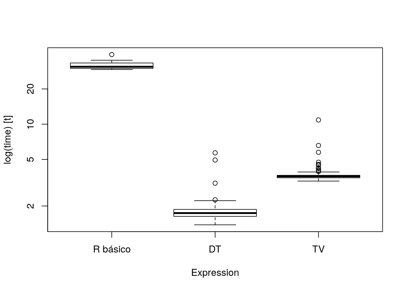

7 >1 estatística para >1 variáveis com >1 estratificadoras

7.1 R básico

tb <- aggregate(cbind(age, balance) ~ marital,
                data = da_bs,
                FUN = function(x) {
                    c(m = mean(x),
                      s = sd(x),
                      n = length(x))
                })
tb

7.2 DT

tb <- da_dt[, list(m = mean(age),
                   s = sd(age),
                   n = length(age)),
            by = marital]
tb

da_dt <- da_dt[, 1:17]
str(da_dt)

tb <- da_dt[, c(lapply(.SD, FUN = mean),
                lapply(.SD, FUN = sd),
                lapply(.SD, FUN = length)),
            by = marital,
            .SDcols = c("age", "balance")]
tb

# Com sulfixo da estatística calculada.
tb <- da_dt[,
            as.list(
                unlist(
                    lapply(X = .SD,
                           FUN = function(x) {
                               list(m = mean(x),
                                    s = sd(x),
                                    n = length(x))
                           })
                )
            ),
            by = marital,
            .SDcols = c("age", "balance")]
tb

7.3 TV

tb <- summarize_at(group_by(da_tv, marital),
                   .vars = c("age", "balance"),
                   .funs = c(m = "mean", s = "sd", n = "length"))
tb

7.4 benchmark

res <- microbenchmark(
    "R básico" = {
        tb <- aggregate(cbind(age, balance) ~ marital,
                        data = da_bs,
                        FUN = function(x) {
                            c(m = mean(x),
                              s = sd(x),
                              n = length(x))
                        })
    },
    "DT" = {
        tb <- da_dt[,
                    as.list(
                        unlist(
                            lapply(X = .SD,
                                   FUN = function(x) {
                                       list(m = mean(x),
                                            s = sd(x),
                                            n = length(x))
                                   })
                        )
                    ),
                    by = marital,
                    .SDcols = c("age", "balance")]
    },
    "TV" = {
        tb <- summarize_at(group_by(da_tv, marital),
                           .vars = c("age", "balance"),
                           .funs = c(m = "mean",
                                     s = "sd",
                                     n = "length"))
    },
    times = 100)
res

## Unit: milliseconds
##      expr       min        lq      mean    median        uq        max
##  R básico 25.168151 25.731104 29.857105 27.183933 29.138981 137.932438
##        DT  1.447232  1.596682  1.712642  1.674132  1.729439   4.908925
##        TV  3.291378  3.511814  3.864821  3.612201  3.828652   8.423800
##  neval cld
##    100   b
##    100  a 
##    100  a

boxplot(res)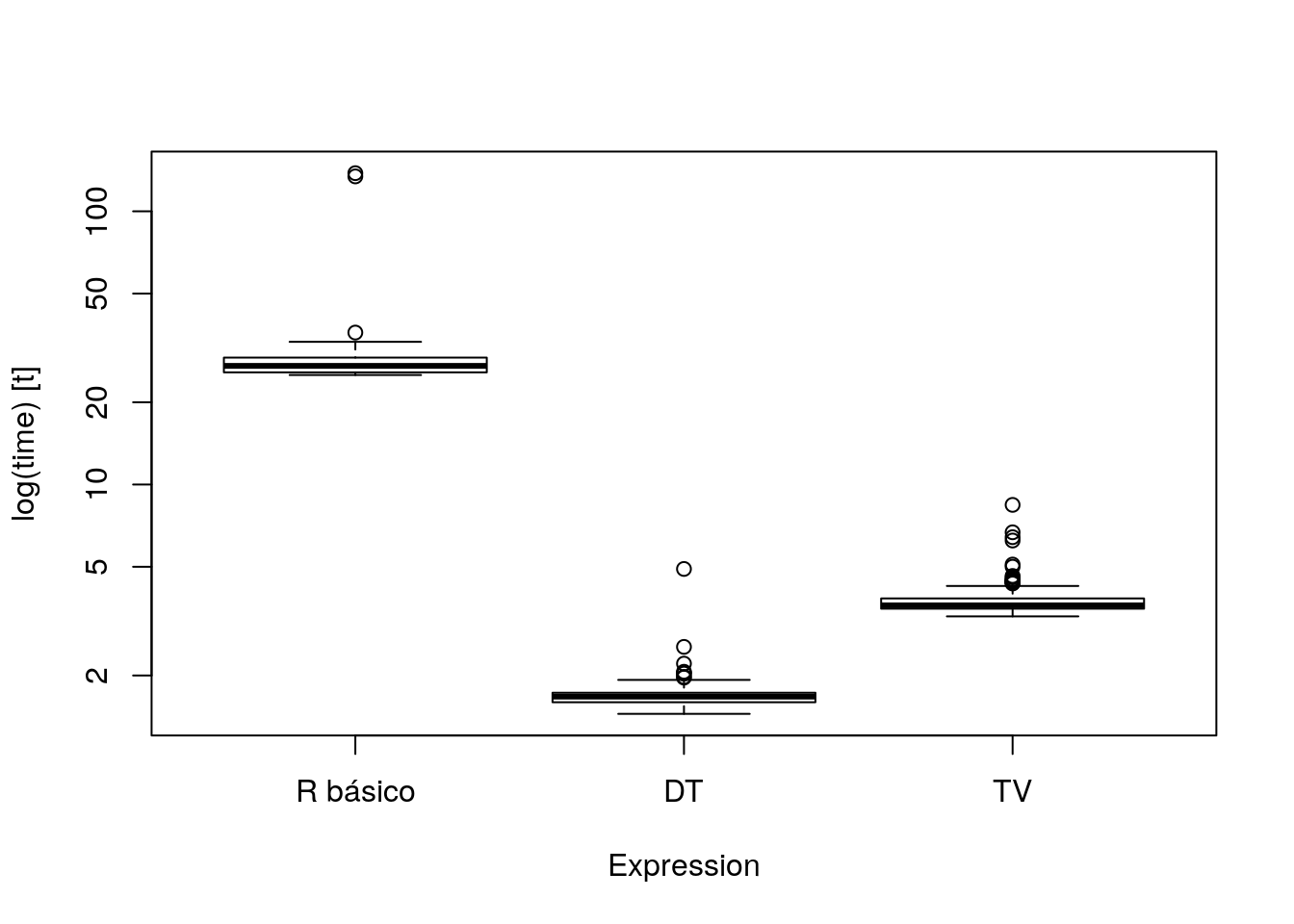

8 Pivotar a tabela

8.1 R básico

tb <- aggregate(duration ~ education + marital + job + housing,
                data = da_bs,
                FUN = mean)
head(tb)

# De long para wide.
tb <- reshape2::dcast(data = tb,
                      formula = education + job + housing ~ marital,
                      value.var = "duration")
str(tb)

# De wide para long.
tb <- reshape2::melt(data = tb,
                     id.vars = 1:3)

8.2 DT

tb <- da_dt[, list(duration = mean(duration)),
            by = list(education, marital, job, housing)]
tb

# De long para wide.
tb <- data.table::dcast(data = tb,
                        formula = education + job + housing ~ marital,
                        value.var = "duration")
str(tb)

# De wide para long.
tb <- data.table::melt(data = tb,
                       id.vars = 1:3)

8.3 TV

tb <- summarize(group_by(da_tv, education, marital, job, housing),
                duration = mean(duration))
tb

# De long para wide.
tb <- spread(data = tb,
             key = "marital",
             value = "duration")
tb

# De wide para long.
tb <- gather(data = tb,
             4:6,
             key = "marital",
             value = "duration")
tb

8.4 benchmark

tb_bs <- aggregate(duration ~ education + marital + job + housing,
                   data = da_bs,
                   FUN = mean)
tb_dt <- da_dt[, list(duration = mean(duration)),
               by = list(education, marital, job, housing)]
tb_tv <- summarize(group_by(da_tv, education, marital, job, housing),
                   duration = mean(duration))

res <- microbenchmark(
    "R básico" = {
        a <- reshape2::dcast(data = tb_bs,
                             formula = education + job + housing ~ marital,
                             value.var = "duration")
        b <- reshape2::melt(data = a, id.vars = 1:3)
    },
    "DT" = {
        a <- data.table::dcast(data = tb_dt,
                               formula = education + job + housing ~ marital,
                               value.var = "duration")
        b <- data.table::melt(data = a, id.vars = 1:3)
    },
    "TV" = {
        a <- spread(data = tb_tv, key = "marital", value = "duration")
        b <- gather(data = a, 4:6, key = "marital", value = "duration")
    },
    times = 300)
res

## Unit: milliseconds
##      expr      min       lq     mean   median       uq       max neval cld
##  R básico 1.304864 1.434951 1.606655 1.518594 1.579854 22.692735   300 a  
##        DT 1.640747 1.806342 1.982913 1.889595 1.996662  6.868913   300  b 
##        TV 3.167120 3.464148 3.724984 3.591237 3.697731 10.143498   300   c

boxplot(res)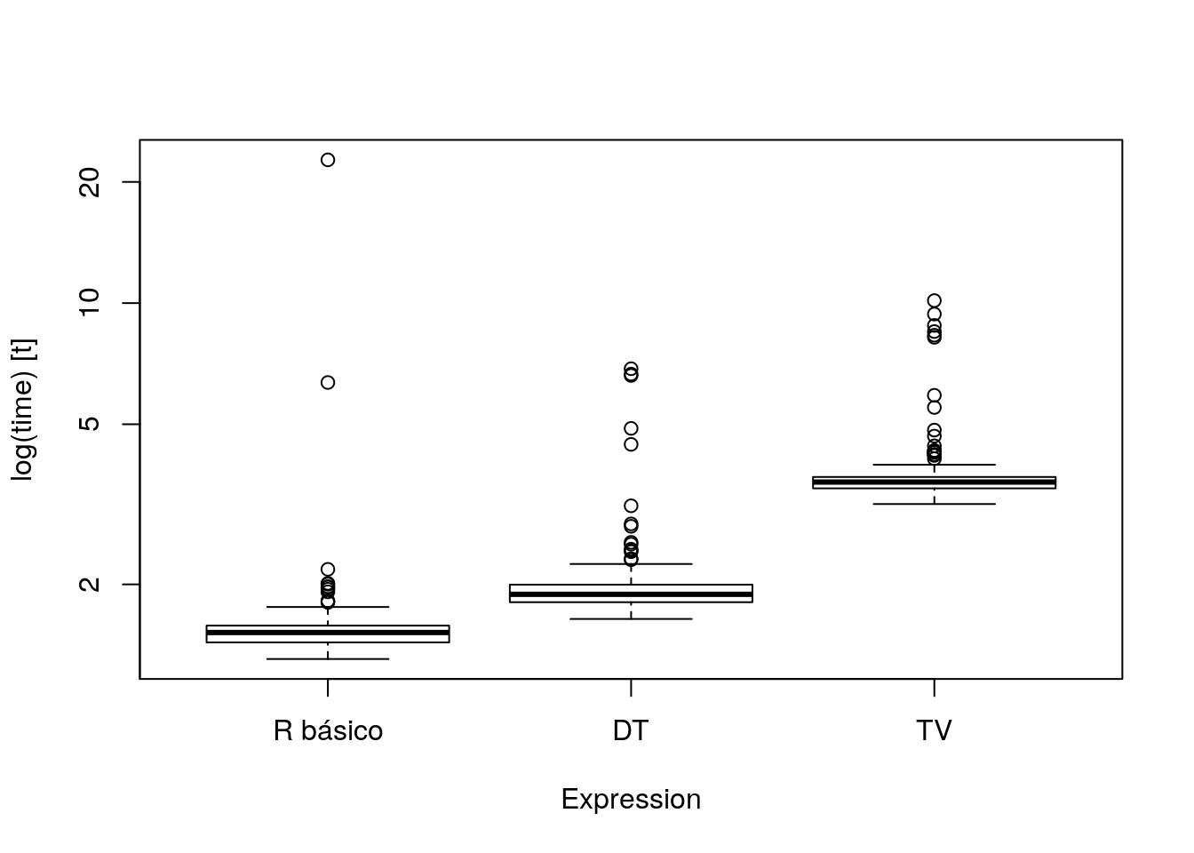

9 Junção de tabelas

9.1 R básico

da_bs <- da_bs[, 1:17]
da_bs$id <- seq_len(nrow(da_bs))
v <- sample(seq_len(ncol(da_bs) - 1), size = 10)

tb1 <- subset(da_bs, select = c(ncol(da_bs), v))
tb2 <- subset(da_bs, select = c(-v))
tb2 <- tb2[sample(seq_len(nrow(da_bs)),
                  size = floor(nrow(da_bs) * 0.7)), ]

# Inner join.
tb <- merge(tb1, tb2)
str(tb)

9.2 DT

da_dt <- da_dt[, 1:17]
da_dt$id <- seq_len(nrow(da_dt))
v <- sample(seq_len(ncol(da_dt) - 1), size = 10)

tb1 <- subset(da_dt, select = c(ncol(da_dt), v))
tb2 <- subset(da_dt, select = c(-v))
tb2 <- tb2[sample(seq_len(nrow(da_dt)),
                  size = floor(nrow(da_dt) * 0.7)), ]

# Inner join.
tb <- merge(tb1, tb2)
str(tb)

# Inner join.
tb <- tb1[tb2, nomatch = 0L, on = "id"]
str(tb)

setkey(tb1, id)
setkey(tb2, id)
tb <- tb1[tb2, nomatch = 0L]
str(tb)

9.3 TV

da_tv <- da_tv[, 1:17]
da_tv$id <- seq_len(nrow(da_tv))
v <- sample(seq_len(ncol(da_tv) - 1), size = 10)

tb1 <- select(da_tv, c(ncol(da_bs), v))
tb2 <- select(da_tv, c(-v))
tb2 <- tb2[sample(seq_len(nrow(da_tv)),
                  size = floor(nrow(da_tv) * 0.7)), ]

tb <- inner_join(tb1, tb2)
str(tb)

9.4 benchmark

tb <- da_dt[, 1:17]
tb <- rbind(tb, tb, tb, tb, tb, tb)
dim(tb)

## [1] 271266     17

tb$id <- seq_len(nrow(tb))
v <- sample(seq_len(ncol(tb) - 1), size = 10)

tb1_bs <- subset(tb, select = c(ncol(tb), v))
tb2_bs <- subset(tb, select = c(-v))
tb2_bs <- tb2_bs[sample(seq_len(nrow(tb)),
                        size = floor(nrow(tb) * 0.7)), ]

tb1_dt <- as.data.table(tb1_bs)
tb2_dt <- as.data.table(tb2_bs)
setkey(tb1_dt, id)
setkey(tb2_dt, id)

tb1_tv <- as_tibble(tb1_bs)
tb2_tv <- as_tibble(tb2_bs)

# c(nrow(tb1_bs), nrow(tb1_dt), nrow(tb1_tv))
# c(nrow(tb2_bs), nrow(tb2_dt), nrow(tb2_tv))
# c(ncol(tb1_bs), ncol(tb1_dt), ncol(tb1_tv))
# c(ncol(tb2_bs), ncol(tb2_dt), ncol(tb2_tv))

res <- microbenchmark(
    "R básico" = {
        tb <- merge(tb1_bs, tb2_bs)
    },
    "DT" = {
        # tb <- merge(tb1_dt, tb2_dt)
        tb <- tb1_dt[tb2_dt, nomatch = 0L]
    },
    "TV" = {
        tb <- suppressMessages(inner_join(tb1_tv, tb2_tv))
    },
    times = 100)
res

## Unit: milliseconds
##      expr       min        lq      mean    median        uq      max neval
##  R básico  40.77013  42.12104  58.81702  46.81349  50.04571 174.1540   100
##        DT  23.71462  24.40274  32.48780  28.55285  30.86476 155.8789   100
##        TV 127.74806 132.55868 145.06705 135.89555 139.89230 295.1353   100
##  cld
##   b 
##  a  
##    c

boxplot(res)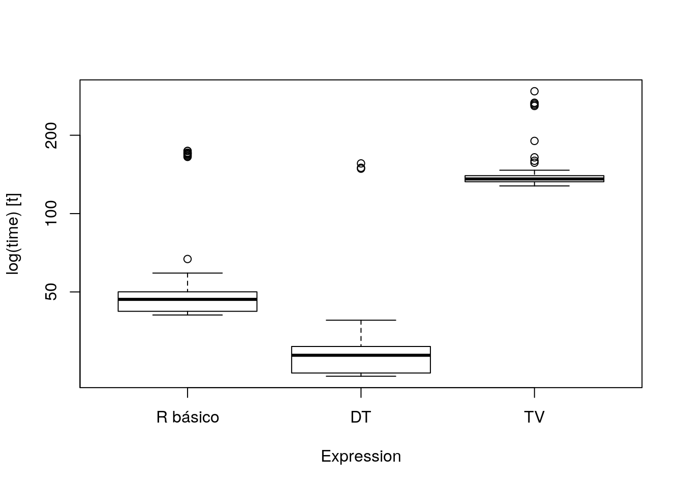

Curso de Especialização em Data Science & Big Data

Linguagens de Programação para Ciência de Dados

Exploração e comunicação de dados com R e Python

Recursos para manipulação de tabelas de dados

Prof. Walmes M. Zeviani

2019-07-31

1 Leitura de arquivo

1.1 R básico

1.2 DT

1.3 TV

1.4 benchmark

2 Ordenar as linhas

2.1 R básico

2.2 DT

2.3 TV

2.4 benchmark

3 Filtros nas linhas

3.1 R básico

3.2 DT

3.3 TV

3.4 benchmark

4 Seleção de variáveis

4.1 R básico

4.2 DT

4.3 TV

4.4 benchmark

5 Transformação de variáveis

5.1 R básico

5.2 DT

5.3 TV

6 1 estatística para >1 variáveis com >1 estratificadoras

6.1 R básico

6.2 DT

6.3 TV

6.4 benchmark

7 >1 estatística para >1 variáveis com >1 estratificadoras

7.1 R básico

7.2 DT

7.3 TV

7.4 benchmark

8 Pivotar a tabela

8.1 R básico

8.2 DT

8.3 TV

8.4 benchmark

9 Junção de tabelas

9.1 R básico

9.2 DT

9.3 TV

9.4 benchmark