7 Bayesian Analysis

Bayesian analysis for Gaussian models is implemented by the function krige.bayes. It can be performed for different "degrees of uncertainty", meaning that model parameters can be treated as ﬁxed or random.

As an example consider a model without nugget and including uncertainty in the mean, sill and range parameters. Prediction at the four locations indicated above is performed by typing a command like:

> bsp4 <- krige.bayes(s100, loc = loci, prior = prior.control(phi.discrete = seq(0,
+ 5, l = 101), phi.prior = "rec"), output = output.control(n.post = 5000))

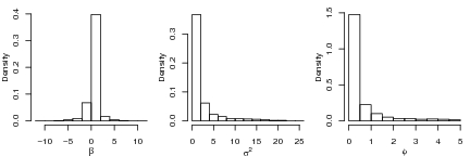
Histograms showing posterior distribution for the model parameters can be plotted by typing:

  > par(mfrow = c(1, 3), mar = c(3, 3, 1, 0.5), mgp = c(2,
  +     1, 0))
  > hist(bsp4$posterior$sample$beta, main = "", xlab = expression(beta),
  +     prob = T)
  > hist(bsp4$posterior$sample$sigmasq, main = "",
  +     xlab = expression(sigma^2), prob = T)
  > hist(bsp4$posterior$sample$phi, main = "", xlab = expression(phi),
  +     prob = T)

pict

Figure 13:

Histograms of samples from posterior distribution

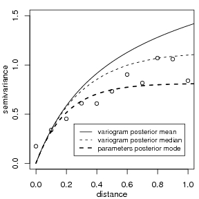
Using summaries of these posterior distributions (means, medians or modes) we can check the "estimated Bayesian variograms" against the empirical variogram, as shown in the next ﬁgure. Notice that it is also possible to compare these estimates with other ﬁtted variograms such as the ones computed in Section 3.

  > plot(bin1, ylim = c(0, 1.5))
  > lines(bsp4, max.dist = 1.2, summ = mean)
  > lines(bsp4, max.dist = 1.2, summ = median, lty = 2)
  > lines(bsp4, max.dist = 1.2, summ = "mode", post = "par",
  +     lwd = 2, lty = 2)
  > legend(0.25, 0.4, legend = c("variogram posterior mean",
  +     "variogram posterior median", "parameters posterior mode"),
  +     lty = c(1, 2, 2), lwd = c(1, 1, 2), cex = 0.8)

pict

Figure 14:

Variogram models based on the posterior distributions

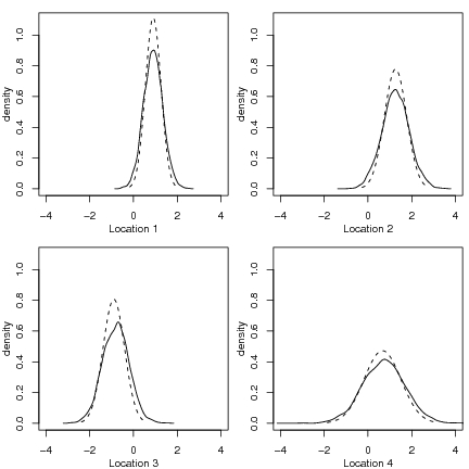
The next ﬁgure shows predictive distributions at the four selected locations. Dashed lines show Gaussian distributions with mean and variance given by results of ordinary kriging obtained in Section 4. The full lines correspond to the Bayesian prediction. The plot shows results of density estimation using samples from the predictive distributions.

  > par(mfrow = c(2, 2))
  > for (i in 1:4) {
  +     kpx <- seq(kc4$pred[i] - 3 * sqrt(kc4$krige.var[i]),
  +         kc4$pred[i] + 3 * sqrt(kc4$krige.var[i]),
  +         l = 100)
  +     kpy <- dnorm(kpx, mean = kc4$pred[i], sd = sqrt(kc4$krige.var[i]))
  +     bp <- density(bsp4$predic$simul[i, ])
  +     rx <- range(c(kpx, bp$x))
  +     ry <- range(c(kpy, bp$y))
  +     plot(cbind(rx, ry), type = "n", xlab = paste("Location",
  +         i), ylab = "density", xlim = c(-4, 4),
  +         ylim = c(0, 1.1))
  +     lines(kpx, kpy, lty = 2)
  +     lines(bp)
  + }

Figure 15:

Predictive distributions at the four selected locations

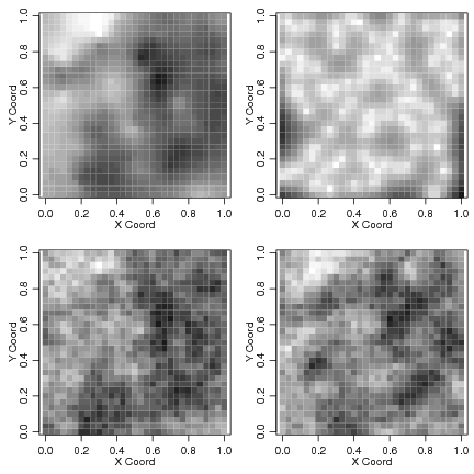
Consider now, under the same model assumptions, obtaining simulations from the predictive distributions on a grid of points covering the area. The commands to deﬁne the grid and perform Bayesian prediction are:

  > pred.grid <- expand.grid(seq(0, 1, l = 31), seq(0,
  +     1, l = 31))
  > bsp <- krige.bayes(s100, loc = pred.grid, prior = prior.control(phi.discrete = seq(0,
  +     5, l = 51)), output = output.control(n.predictive = 2))

Maps with the summaries and simulations of the predictive distribution can be plotted as follows.

  > par(mfrow = c(2, 2), mar = c(3, 3, 1, 0.5), mgp = c(1.5,
  +     0.7, 0))
  > image(bsp, loc = pred.grid, main = "predicted",
  +     col = gray(seq(1, 0.1, l = 30)))
  > image(bsp, val = "variance", loc = pred.grid,
  +     main = "prediction variance", col = gray(seq(1,
  +         0.1, l = 30)))
  > image(bsp, val = "simulation", number.col = 1,
  +     loc = pred.grid, main = "a simulation from\nthe predictive distribution",
  +     col = gray(seq(1, 0.1, l = 30)))
  > image(bsp, val = "simulation", number.col = 2,
  +     loc = pred.grid, main = "another simulation from \n the predictive distribution",
  +     col = gray(seq(1, 0.1, l = 30)))

pict

Figure 16:

Maps obtained from the predictive distribution