4 Parameter Estimation
Theoretical and empirical variograms can be plotted and visually compared. For example, the
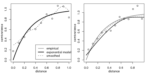
left panel in Figure 6 shows the theoretical variogram model used to simulate the data s100 and
two estimated variograms.
> bin1 <- variog(s100, uvec = seq(0, 1, l = 11))
> plot(bin1)
> lines.variomodel(cov.model = "exp", cov.pars = c(1,
+ 0.3), nugget = 0, max.dist = 1, lwd = 3)
> smooth <- variog(s100, option = "smooth", max.dist = 1,
+ n.points = 100, kernel = "normal", band = 0.2)
> lines(smooth, type = "l", lty = 2)
> legend(0.4, 0.3, c("empirical", "exponential model",
+ "smoothed"), lty = c(1, 1, 2), lwd = c(1,
+ 3, 1))
In practice we usually don’t know the true parameters which have top be estimated by some
method. In the package geoR the model parameters can be estimated:
- “by eye”: trying different models over empirical variograms (using the function
lines.variomodel),
- by least squares fit of empirical variograms: with options for ordinary (OLS) and
weighted (WLS) least squares (using the function variofit),
- by likelihood based methods: with options for maximum likelihood (ML) and restricted
maximum likelihood (REML) (using the function likfit),
- Bayesian methods: are also implemented and will be presented in Section 5 (using
the function krige.bayes).
Fitting “by eye” consists of drawing curves of theoretical variogram functions over an
empirical variogram, changing the variogram model and/or its parameters and, at last, choosing
one of them. The following commands show how to add a line with a variogram model to a
variogram plot. Three different variogram models are used.
> plot(variog(s100, max.dist = 1))
> lines.variomodel(cov.model = "exp", cov.pars = c(1,
+ 0.3), nug = 0, max.dist = 1)
> lines.variomodel(cov.model = "mat", cov.pars = c(0.85,
+ 0.2), nug = 0.1, kappa = 1, max.dist = 1,
+ lty = 2)
> lines.variomodel(cov.model = "sph", cov.pars = c(0.8,
+ 0.8), nug = 0.1, max.dist = 1, lwd = 2)
When using the parameter estimation functions variofit and likfit the nugget effect
parameter can either be estimated or set to a fixed value. The same applies for smoothness,
anisotropy and transformation parameters. Options for taking trends into account are also
included. Trends can be specified as polynomial functions of the coordinates and/or linear
functions of given covariates.
An example call to likfit is given below. Methods for print() and summary() have been
written to summarize the resulting objects.
> ml <- likfit(s100, ini = c(1, 0.5))
---------------------------------------------------------------
likfit: likelihood maximisation using the function optim.
likfit: Use control() to pass additional
arguments for the maximisation function.
For further details see documentation for optim.
likfit: It is highly advisable to run this function several
times with different initial values for the parameters.
likfit: WARNING: This step can be time demanding!
---------------------------------------------------------------
likfit: end of numerical maximisation.
likfit: estimated model parameters:
beta tausq sigmasq phi
"0.7766" "0.0000" "0.7517" "0.1827"
likfit: maximised log-likelihood = -83.57
Summary of the parameter estimation
-----------------------------------
Estimation method: maximum likelihood
Parameters of the mean component (trend):
beta
0.7766
Parameters of the spatial component:
correlation function: exponential
(estimated) variance parameter sigmasq (partial sill) = 0.7517
(estimated) cor. fct. parameter phi (range parameter) = 0.1827
anisotropy parameters:
(fixed) anisotropy angle = 0 ( 0 degrees )
(fixed) anisotropy ratio = 1
Parameter of the error component:
(estimated) nugget = 0
Transformation parameter:
(fixed) Box-Cox parameter = 1 (no transformation)
Maximised Likelihood:
log.L n.params AIC BIC
"-83.57" "4" "175.1" "185.6"
non spatial model:
log.L n.params AIC BIC
"-125.8" "2" "255.6" "260.8"
Call:
likfit(geodata = s100, ini.cov.pars = c(1, 0.5))
The commands below shows how to fit models by using different methods, with options for
fixed or estimated nugget parameter. Notice there are other features not illustrated here such as
estimation of trends, anisotropy, smoothness and Box-Cox transformation parameter. Notice in
the call above that the functions show some messages while they are running — and we don’t
want to see them in the following calls. To prevent this we can set the argument messages =
FALSE at each function call or, to set it globally for all functions use options() as
follows.
> options(geoR.messages = FALSE)
- Fitting models with nugget fixed to zero
> ml <- likfit(s100, ini = c(1, 0.5), fix.nugget = T)
> reml <- likfit(s100, ini = c(1, 0.5), fix.nugget = T,
+ method = "RML")
> ols <- variofit(bin1, ini = c(1, 0.5), fix.nugget = T,
+ weights = "equal")
> wls <- variofit(bin1, ini = c(1, 0.5), fix.nugget = T)
- Fitting models with a fixed value for the nugget
> ml.fn <- likfit(s100, ini = c(1, 0.5), fix.nugget = T,
+ nugget = 0.15)
> reml.fn <- likfit(s100, ini = c(1, 0.5), fix.nugget = T,
+ nugget = 0.15, method = "RML")
> ols.fn <- variofit(bin1, ini = c(1, 0.5), fix.nugget = T,
+ nugget = 0.15, weights = "equal")
> wls.fn <- variofit(bin1, ini = c(1, 0.5), fix.nugget = T,
+ nugget = 0.15)
- Fitting models estimated nugget
> ml.n <- likfit(s100, ini = c(1, 0.5), nug = 0.5)
> reml.n <- likfit(s100, ini = c(1, 0.5), nug = 0.5,
+ method = "RML")
> ols.n <- variofit(bin1, ini = c(1, 0.5), nugget = 0.5,
+ weights = "equal")
> wls.n <- variofit(bin1, ini = c(1, 0.5), nugget = 0.5)
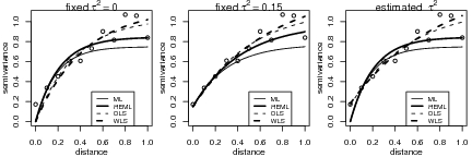
Now, the comands for plotting fitted models against empirical variogram as show in Figure 4
are:
> par(mfrow = c(1, 3))
> plot(bin1, main = expression(paste("fixed ", tau^2 ==
+ 0)))
> lines(ml, max.dist = 1)
> lines(reml, lwd = 2, max.dist = 1)
> lines(ols, lty = 2, max.dist = 1)
> lines(wls, lty = 2, lwd = 2, max.dist = 1)
> legend(0.5, 0.3, legend = c("ML", "REML", "OLS",
+ "WLS"), lty = c(1, 1, 2, 2), lwd = c(1, 2,
+ 1, 2), cex = 0.7)
> plot(bin1, main = expression(paste("fixed ", tau^2 ==
+ 0.15)))
> lines(ml.fn, max.dist = 1)
> lines(reml.fn, lwd = 2, max.dist = 1)
> lines(ols.fn, lty = 2, max.dist = 1)
> lines(wls.fn, lty = 2, lwd = 2, max.dist = 1)
> legend(0.5, 0.3, legend = c("ML", "REML", "OLS",
+ "WLS"), lty = c(1, 1, 2, 2), lwd = c(1, 2,
+ 1, 2), cex = 0.7)
> plot(bin1, main = expression(paste("estimated ",
+ tau^2)))
> lines(ml.n, max.dist = 1)
> lines(reml.n, lwd = 2, max.dist = 1)
> lines(ols.n, lty = 2, max.dist = 1)
> lines(wls.n, lty = 2, lwd = 2, max.dist = 1)
> legend(0.5, 0.3, legend = c("ML", "REML", "OLS",
+ "WLS"), lty = c(1, 1, 2, 2), lwd = c(1, 2,
+ 1, 2), cex = 0.7)
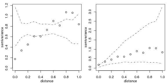
Two kinds of variogram envelopes computed by simulation are illustrated in the figure
below.
The plot on the left-hand side shows an envelope based on permutations of the data values
across the locations, i.e. envelopes built under the assumption of no spatial correlation. The
envelopes shown on the right-hand side are based on simulations from a given set of model
parameters, in this example the parameter estimates from the WLS variogram fit. This envelope
shows the variability of the empirical variogram.
> env.mc <- variog.mc.env(s100, obj.var = bin1)
> env.model <- variog.model.env(s100, obj.var = bin1,
+ model = wls)
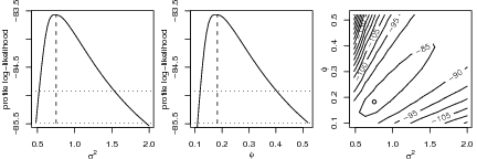
Profile likelihoods (1-D and 2-D) are computed by the function proflik. Here we show the
profile likelihoods for the covariance parameters of the model without nugget effect previously
fitted by likfit.
WARNING: RUNNING THE NEXT COMMAND CAN BE TIME-CONSUMING