Number of Bolls in Cotton under Artifitial Defoliation

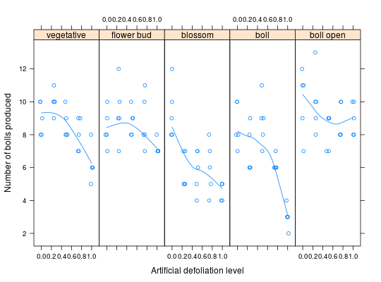
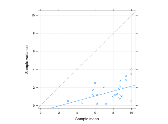
These data are the results of a greenshouse factorial experiment performed to evaluate the effect of defoliation on the production of cotton at different growth stages. The experiment is a \(5\times 5\) factorial with 5 replications in a complete randomized design. The experimental unit was a pot with 2 cotton plants. The response variable is the number of bolls produced at the end of the crop cycle. The observed number of cotton bolls is a count variable with underdispersion (sample variance less than the sample mean).

Format

A data.frame with 125 records and 4 variables, described below.

• defol A numeric factor with 5 levels that represents the (artifitial) levels of defoliation (percent in leaf area removed with scissors) applied for all leaves of the plants.

• phenol A categorical ordered factor with 5 levels that represents the (phenological) growth stages of the cotton plants in which the levels of defoliation was applied.

• rept Integer variable that indexes each experimenal unit in each treatment cell.

• bolls The number of bolls produced (count variable) evaluated at harvest of cotton.

References

Silva, A. M., Degrande, P. E., Suekane, R., Fernandes, M. G., Zeviani, W. M. (2012). Impacto de diferentes níveis de desfolha artificial nos estádios fenológicos do algodoeiro. Revista de Ciências Agrárias, 35(1), 163–172. http://www.scielo.mec.pt/pdf/rca/v35n1/v35n1a16.pdf.

Zeviani, W. M., Ribeiro, P. J., Bonat, W. H., Shimakura, S. E., Muniz, J. A. (2014). The Gamma-count distribution in the analysis of experimental underdispersed data. Journal of Applied Statistics, 41(12), 1–11. http://doi.org/10.1080/02664763.2014.922168, http://leg.ufpr.br/doku.php/publications:papercompanions:zeviani-jas2014.

Examples

library(lattice)
library(latticeExtra)
#> Loading required package: RColorBrewer

data(cotton_defol)
str(cotton_defol)
#> 'data.frame':	125 obs. of  4 variables:
#>  $ phenol: Factor w/ 5 levels "vegetative","flower bud",..: 1 1 1 1 1 1 1 1 1 1 ...
#>  $ defol : num  0 0 0 0 0 0.25 0.25 0.25 0.25 0.25 ...
#>  $ rept  : int  1 2 3 4 5 1 2 3 4 5 ...
#>  $ bolls : num  10 9 8 8 10 11 9 10 10 10 ...

# x11(width = 7, height = 2.8)
xyplot(bolls ~ defol | phenol,
       data = cotton_defol,
       layout = c(NA, 1),
       type = c("p", "smooth"),
       xlab = "Artificial defoliation level",
       ylab = "Number of bolls produced",
       xlim = extendrange(c(0:1), f = 0.15),
       jitter.x = TRUE)

# Sample mean and variance in each treatment cell.
mv <- aggregate(bolls ~ phenol + defol,
                data = cotton_defol,
                FUN = function(x) {
                    c(mean = mean(x), var = var(x))
                })
str(mv)
#> 'data.frame':	25 obs. of  3 variables:
#>  $ phenol: Factor w/ 5 levels "vegetative","flower bud",..: 1 2 3 4 5 1 2 3 4 5 ...
#>  $ defol : num  0 0 0 0 0 0.25 0.25 0.25 0.25 0.25 ...
#>  $ bolls : num [1:25, 1:2] 9 8.4 9.4 8.6 10 10 9.4 5.8 7 10 ...
#>   ..- attr(*, "dimnames")=List of 2
#>   .. ..$ : NULL
#>   .. ..$ : chr  "mean" "var"

xlim <- ylim <- extendrange(c(mv$bolls), f = 0.05)

# Evidence of underdispersion.
xyplot(bolls[, "var"] ~ bolls[, "mean"],
       data = mv,
       grid = TRUE,
       aspect = "iso",
       type = c("p", "r"),
       xlim = xlim,
       ylim = ylim,
       ylab = "Sample variance",
       xlab = "Sample mean") +
    layer(panel.abline(a = 0, b = 1, lty = 2))