Working with sp and aRT
Pedro R. Andrade
Paulo Justiniano Ribeiro Júnior
July 20, 2009
Contents
1 Introduction
sp (Pebesma & Bivand, 2005) is an important package that defines standards and
allows for exchanging information between spatial packages in R. As aRT manipulates
all spatial data formats, it was designed to follow sp standards to represent spatial
data, storing and retrieving data using the sp format. Therefore, when working with
aRT and spatial data in R it is required that objects containing spatial data are
converted, whenever necessary, to the sp format. For futher details on sp package
see http://r-spatial.sourceforge.net.
On the other hand, TerraLib databases can contain data that cannot be directly
converted to sp data. For example:
- TerraLib (and therefore aRT) requires ID in all spatial data, different from
sp, that requires ID only for lines and polygons.
- TerraLib layers have support to multigeometry, meaning that each spatial
element can have more than one geometry associated. For example, a layer
of cities can store both contours and centroids.
- geometries and attributes are stored in different objects in a
TerraLib database. Geometries are stored directly inside layers, whereas
attributes are stored in tables inside layers. The reason why tables cannot
be in the same object as geometries is because TerraLib supports different
table formats, for example static, event, and dynamic.
This document illustrates how to manipulate spatial data in aRT, showing
how to import to and read from TerraLib databases. The data (and also
some sentences!) of this document are extracted from Pebesma and Bivand
(2005).
We start by loading the package and, for convenience here, setting aRT to the
silent mode which hides some information messages issued by aRT functions; followed
by establishing a connection to a DBMS. The database to be used in the
examples is called “sp”, which, if exists, is removed from the DBMS and
recreated. Notice this is a TerraLibdatabase, i.e., a database created following the
TerraLib structure.
> require(aRT)
> aRTsilent(TRUE) # hiding info messages
> con = openConn(name="default")
> if(any(showDbs(con)=="sp")) deleteDb(con, "sp", force=T)
> db = createDb(con, "sp")
Further details on connections to the DBMS are provided by the vignette
aRTconn.
2 Spatial points
2.1 Points without attributes
Our first example illustrates how to handle data with a points geometry. For instance,
consider a set of 10 points randomly generated on the unit square [0,1] × [0,1] and
stored in a matrix xy. The first step is to use sp to convert into a SpatialPoints
object.
> xy = matrix(runif(20), nc=2)
> xy.sp = SpatialPoints(xy)
> xy.sp
SpatialPoints:
coords.x1 coords.x2
[1,] 0.6739453 0.3021973
[2,] 0.9619853 0.6170330
[3,] 0.9228386 0.9050982
[4,] 0.7747456 0.8476483
[5,] 0.7248062 0.4579902
[6,] 0.7413480 0.3863993
[7,] 0.6302933 0.6443511
[8,] 0.1903071 0.7170724
[9,] 0.6977443 0.1980982
[10,] 0.3703263 0.2772779
Coordinate Reference System (CRS) arguments: NA
However, an SpatialPoints object cannot be used by aRT functions because it does not
have ID and it is necessary to convert to a SpatialPointsDataFrame.
> xy.spdf = SpatialPointsDataFrame(xy, data.frame(ID=paste(1:10)))
Note that here you can use both xy or xy.spdf as argument to Spatial
PointsDataFrame.
The first step to store this data in a TerraLib database is to create a layer. A layer
is a container that can store any geometric type and also, optionally, other types of
objects. A layer can be created in a database using createLayer() and the function
call receives as arguments the database object and a string defining the name to be
set for the layer.
> lpoints = createLayer(db, "points")
> lpoints
Object of class aRTlayer
Layer: "points"
Database: "sp"
Layer is empty
Projection Name: "NoProjection"
Projection Datum: "Spherical"
Tables: (none)
Notice that we have two names, "points" which is the name of the layer in the
database, and lpoints, an R object which can access "points". Next the
function addPoints() is used to store the points into the layer. Notice that
after that the layer object acknowledges the points are now stored into the
database.
> addPoints(lpoints, xy.spdf)
> lpoints
Object of class aRTlayer
Layer: "points"
Database: "sp"
Number of points: 10
Projection Name: "NoProjection"
Projection Datum: "Spherical"
Tables: (none)
To conclude storing the points a further step creating adding a table to the layer is
still necessary in order to ba able to read any data from the layer. This is a
TerraLib requirement needed even when the spatial data does not have any
attributes. Geometries with no entry in any table cannot be retrieved from the
database.
> tpoints = createTable(lpoints, "tpoints")
> tpoints
Object of class aRTtable
Table: "tpoints"
Type: static
Layer: "points"
Rows: 10
Attributes:
id: character[16] (key)
Object of class aRTlayer
Layer: "points"
Database: "sp"
Number of points: 10
Projection Name: "NoProjection"
Projection Datum: "Spherical"
Tables:
"tpoints": static
Now the layer has 10 points and one table, and we can retrieve the point coordinates
using getPoints(), which returns an object of class SpatialPointsDataFrame:
> points = getPoints(lpoints)
> points
coordinates ID
1 (0.673945, 0.302197) 1
2 (0.370326, 0.277278) 10
3 (0.961985, 0.617033) 2
4 (0.922839, 0.905098) 3
5 (0.774746, 0.847648) 4
6 (0.724806, 0.45799) 5
7 (0.741348, 0.386399) 6
8 (0.630293, 0.644351) 7
9 (0.190307, 0.717072) 8
10 (0.697744, 0.198098) 9
Note that the points have a different order from the original data. That is
because the database stores the IDs as characters, therefore 10 comes before
2.
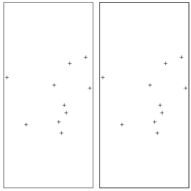
Figure 2 illustrates two different ways for visualising the point coordinates, on the
left by plotting the points from an R object with plot(points), or directly from the
layer, with plot(lpoints), which does not requires the existence of an R object
containing the points.
2.2 Points with attributes
Another possible way of creating a SpatialPointsDataFrame object is by building it
by combining a SpatialPoints object and a data frame containing associated
attributes. In the following example we combine the object xy.sp with a data
frame df containg attributes. Notice the ID column is required by any sp
object.
> df = data.frame(z1 = round(5 + rnorm(10), 2), z2 = 0:9, ID = paste(1:10))
> xy.spdf = SpatialPointsDataFrame(xy.sp, df)
> xy.spdf
coordinates z1 z2 ID
1 (0.673945, 0.302197) 3.10 0 1
2 (0.961985, 0.617033) 4.15 1 2
3 (0.922839, 0.905098) 3.68 2 3
4 (0.774746, 0.847648) 4.45 3 4
5 (0.724806, 0.45799) 6.62 4 5
6 (0.741348, 0.386399) 5.57 5 6
7 (0.630293, 0.644351) 3.66 6 7
8 (0.190307, 0.717072) 3.75 7 8
9 (0.697744, 0.198098) 5.19 8 9
10 (0.370326, 0.277278) 5.02 9 10
As before we create a layer and aad the points to it. Next, as our object now has
attributes, we can import the table data using importTable().
> lpointsdf = createLayer(db, "lpointsdf")
> addPoints(lpointsdf, xy.spdf)
> tpointsdf = importTable(lpointsdf, "tpointsdf", ID="ID", xy.spdf)
> tpointsdf
Object of class aRTtable
Table: "tpointsdf"
Type: static
Layer: "lpointsdf"
Rows: 10
Attributes:
id: character[16] (key)
z1: numeric
z2: integer
Object of class aRTlayer
Layer: "lpointsdf"
Database: "sp"
Number of points: 10
Projection Name: "NoProjection"
Projection Datum: "Spherical"
Tables:
"tpointsdf": static
When retrieving data from the database to R getting point coordinates and the
table at once from the layer we can use a second argument of getPoints() with the
table to be read.
> getPoints(lpointsdf, tpointsdf)
coordinates ID z1 z2
1 (0.673945, 0.302197) 1 3.10 0
2 (0.370326, 0.277278) 10 5.02 9
3 (0.961985, 0.617033) 2 4.15 1
4 (0.922839, 0.905098) 3 3.68 2
5 (0.774746, 0.847648) 4 4.45 3
6 (0.724806, 0.45799) 5 6.62 4
7 (0.741348, 0.386399) 6 5.57 5
8 (0.630293, 0.644351) 7 3.66 6
9 (0.190307, 0.717072) 8 3.75 7
10 (0.697744, 0.198098) 9 5.19 8
2.3 Doing all at once
All the steps above can be encapsulated using importSpData().
3 Grids
(not supported yet)
4 Lines
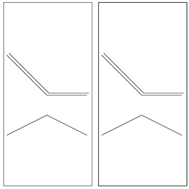
4.1 Building line objects from scratch
In many instances, line coordinates will be retrieved from external sources. The
following example shows how to build an object of class SpatialLines from scratch.
As objects from this class already stores ID, they are pushed in the layer directly
using addLines().
> l1 = cbind(c(1,2,3),c(3,2,2))
> l1a = cbind(l1[,1]+.05,l1[,2]+.05)
> l2 = cbind(c(1,2,3),c(1,1.5,1))
> Sl1 = Line(l1)
> Sl1a = Line(l1a)
> Sl2 = Line(l2)
> #S1 = Lines(list(Sl1, Sl1a), ID="a")
> S1 = Lines(list(Sl1), ID="a")
> S2 = Lines(list(Sl2), ID="b")
> S3 = Lines(list(Sl1a), ID="c")
> Sl = SpatialLines(list(S1,S2,S3))
> llines = createLayer(db,"llines")
> addLines(llines, Sl)
> createTable(llines, "llines")
Object of class aRTtable
Table: "llines"
Type: static
Layer: "llines"
Rows: 3
Attributes:
id: character[16] (key)
4.2 Building line objects with attributes
The same as polygons
5 Polygons
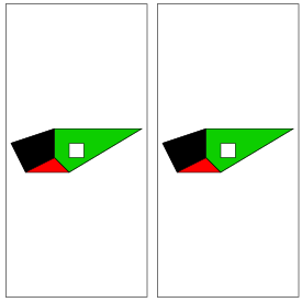
5.1 Building from scratch
The following example shows how a set of polygons are built from scratch. Note that
Sr4 has the opposite direction (right) as the other three; it is meant to represent a
hole in the Sr3 polygon.
> #genPol = function(quant)
> #{
> # res = list()
> # res = lapply(1:quant, function(x) {
> # from = round(runif(2,1,20),2)
> # to = from + round(runif(2,1,5),2)
> #
> # Sr1 = Polygon(cbind(c(from[1],from[1],to[1],to[1], from[1]),
> # c(from[2],to[2], to[2],from[2],from[2])))
> # Srs1 = Polygons(list(Sr1),paste(x))
> # })
> # SR = SpatialPolygons(res, 1:quant)
> #}
>
> Sr1 = Polygon(cbind(c(2,4,4,1,2),c(2,3,5,4,2)))
> Sr2 = Polygon(cbind(c(5,4,2,5),c(2,3,2,2)))
> Sr3 = Polygon(cbind(c(4,4,5,10,4),c(5,3,2,5,5)))
> Sr4 = Polygon(cbind(c(5,6,6,5,5),c(4,4,3,3,4)), hole = TRUE)
> Srs1 = Polygons(list(Sr1), "s1")
> Srs2 = Polygons(list(Sr2), "s2")
> Srs3 = Polygons(list(Sr3, Sr4), "s3/4")
> SR = SpatialPolygons(list(Srs1,Srs2,Srs3), 1:3)
> lrings = createLayer(db, "lrings")
> addPolygons(lrings, SR)
> trings = createTable(lrings, "trings")
> #th=createTheme(lrings, "trings")
> lrings
Object of class aRTlayer
Layer: "lrings"
Database: "sp"
Number of polygons: 4
Projection Name: "NoProjection"
Projection Datum: "Spherical"
Tables:
"trings": static
> #sr = as.SpatialPolygon(getGeometry(lrings))
>
> pols = getPolygons(lrings)
5.2 Polygons with attributes
Polygons with attributes, objects of class SpatialPolygonsDataFrame, are built from
the SpatialPolygons object (topology) and the attributes (data.frame):
> #attr = data.frame(a=1:3, b=3:1, row.names=c("s1","s2","s3/4"))
> #SrDf = SpatialPolygonsDataFrame(SR, attr)
> #lringsdf = createLayer(db, "lringsdf")
> #addPolygons(lringsdf, SrDf)
To import the attributes, we need to create a table, but, due to the internal
differences of sp data storage
> #xy.spdf@data
> #SrDf@data
> #class(SrDf@data)
we need to insert SrDf manually, creating both table and the two integer columns before
inserting the data:
> #tringsdf = createTable(lringsdf, "tringsdf", ID="ID", gen=F)
> #createColumn(tringsdf, "a", "i")
> #createColumn(tringsdf, "b", "i")
> #addRows(tringsdf, SrDf@data)
> #tringsdf
> #lringsdf
>
> #getData(tringsdf)
>
> #sr = as.SpatialPolygons(getGeometry(lringsdf))
> #summary(sr)
> #sr = as.SpatialPolygonsDataFrame(getGeometry(lringsdf))
> #sr
References
-
- Chambers, J.M., 1998, Programming with data, a guide to the S language.
Springer, New York.
-
- Pebesma, E.J. and Bivand, R.S., 2005, Classes and methods for spatial data
in R, R-News 5 (2), pp. 9-13.