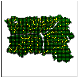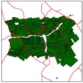
Figure 1: Database that will be used to compute spatial relations.
This vignette describes how to create Generalized Proximity Matrixes (GPM) within aRT. GPM is based on the idea that Euclidean spaces are not enough to describe the relations that take place within the geographical space. For more information on GPM, see Aguiar et al. (2003); Modeling Spatial Relations by Generalized Proximity Matrices. Proceedings of V Brazilian Symposium in Geoinformatics (GeoInfo’03).
GPM is composed by a set of strategies that try to capture such spatial warp, computing operations over sets of spatial data. Some strategies have been implemented within aRT. In the next sections, we will describe the basic structure of the implementation and present some examples of creating proximity matrixes. Before starting, we will read some spatial data.
The database, shown in Figure 1, contains:
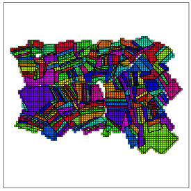
From the set of polygons, we create a set of points with their centroids and a layer of cells, shown in Figure 2.
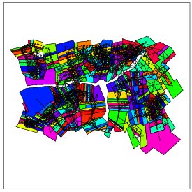
The first example of GPM starts with a strategy that uses the intersection area to create relations between cells and polygons. A cell is connected to the polygon that has the largest intersection area. connectToBiggerIntersectionArea() can be used to compute this operation. It gets a set of cells and a layer of polygons as arguments and returns a table with two columns: the object id of the polygon with largest intersection area and the intersection area itself.
After creating the function that generates the neighbors of a given object, the GPM can be created straightforwardly by calling createGPM(). It takes two arguments: the database layer with the dataset and the function that creates the neighborhood. The GPM stores the neighborhoods of all objects, with other atributes according to the adopted strategy, such as the ‘area,’ in this case.
This GPM, shown in Figure 3, can be saved as a .gpm, GAL or GWT file by using saveGPM(), presented in more details in section 8. The code below saves it in a .gpm file:
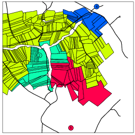
The second strategy uses the centroids to create relations between points that are closer than 1000m. To accomplish that, we use getNeighborsMaxDistanceFunction() to generate a function that returns the neighbors within a given distance. Finally we use createGPM() from the layer of polygons to generate the results shown in Figure 4.
The strategy presented in this section computes neighborhoods based on the intersection between lines and cells. Each cell is connected with the line segments that intersects it. The function getNeighborsIntersectionLines() can be used to generate the function that returns the neighbor lines that intersects a given cell. It gets a layer of cells and a layer of lines as arguments and returns a function used to effectively create the GPM. Finally, the GPM is effectively created by the createGPM(), which receives as arguments the layer of cells passed as argument in the getNeighborsIntersectionLines() fuction, and the result returned by it. The code below creates a neighborhood between the layer "cells" and the layer "rodovias".
This GPM can be saved in a file (.gpm, .GAL or .GWT) through the saveGPM() method, presented in section 8.
In this section, we present a function that computes neighborhoods between a layer of cells and a layer of points based on the "contains" spatial relation. Thus, a cell is connected to the points located inside its area. The function getNeighborsContainedPoints generates the function that returns the neighbor points located inside the area of a given cell. It gets a layer of cells and a layer of points as arguments and returns a function used to effectively compute the GPM. Finally, the GPM is effectively created by the createGPM() method, which receives as arguments the layer of cells passed as argument in the getNeighborsContainedPoints() function, and the result returned by it. The code below creates a neighborhood between the layer "cells" and the layer "comunidades".
This GPM can be saved in a file (.gpm, .GAL or .GWT) through the saveGPM() method, presented in section 8.
In this section, we present an strategy to compute neighborhoods between a layer of lines and a layer of polygons, in which each line has as neighbors the polygons intersected by it. The function connectLineToIntersectionPolygons() generates the function that returns the neighbor polygons intersected by a given line. It gets a layer of lines and a layer of polygons as arguments and returns a function used to effectively compute the GPM. Finally, the GPM is effectively created by the createGPM() method, which receives as arguments the layer of lines passed as argument in the connectLineToIntersectionPolygons() function, and the result returned by it. The code below creates a neighborhood between the layer "rodovias" and the layer "lotes".
The last strategy presented in this vignette computes neighborhoods based on the distance through a given network represented by a set of lines. The original data has to be very well represented, with the starting and ending points of two lines being connected to one another when they share the same position in space. In this type of network, it is possible to enter and leave the roads in any position. createOpenNetwork() is then used to generate the network. It takes as arguments the destination (reference) points, the lines that will be used to represent the network, and a function that computes the distance on the network given the length of the lines and their id. The code below creates a network that reduces the distance within the network by one fifth of the Euclidean distance for paved roads and by half on the others. The attribute pavimentada of the table connected to the layer of lines indicates whether the road is paved or not.
Figure 5 shows the polygons drawn with the color of the closest point through the network. There is a current known limitation in the current version of createOpenNetwork(), that does not work properly when the entry point on the network for a given point is the start or end of a line segment.
Once we have created the GPM through one of the strategies presented above, we can save it in a file, which can be a GPM file (".gpm"), a GAL file (".gal" or ".GAL") or a GWT file (".gal" or ".GWT"), through the function saveGPM(). The arguments of this function are:
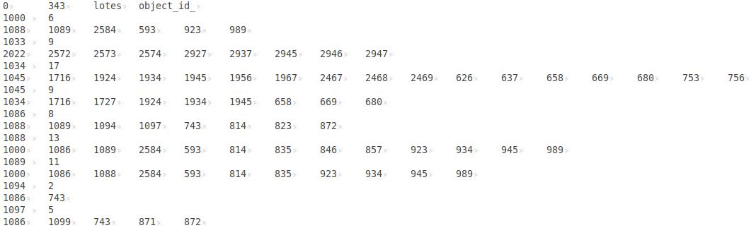
The code below saves the GPM gpmnetwork, created in section 7 in the file "gpmnetwork.gpm", presented in Figure 6.
The structure of the GPM file is presented in Table 1. The first line is the header, and the GPM starts in the second line. In the header, we have the following fields:
From the second line until the end of the file, the GPM is represented. The neighborhood of each object is represented in two lines. The first contains:
and the second contais the neighborhood of the object which ID is in the previous line, represented by the fields below, following the structure presented in Table 1:
The structure of the GAL file is presented in Table 2. It does not store informations about the attributes of the GPM, but only if two objects are neighbors or not. Furthermore, it does not support neighborhoods between objects of different layers. The first line of the file, as well as in the GPM file, is the header, and the GPM starts in the second line. In the header, we have the following fields:
From the second line until the end of file, the relations are represented. The neighborhood of each object is represented in two lines. The first contains:
and the second line contains the unique identifier of the neighbors
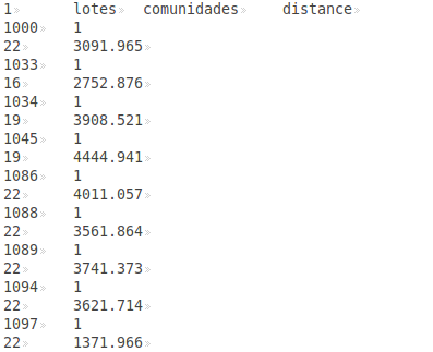
(ID_Neighbor_M) of the N-th object. The code below saves the GPM gpmdistance,
created in section 3, in the file "gpmdistance.GAL", presented in Figure
7.
The structure of the GWT file is presented in Table 3. It can store one of the attributes of the GPM, which name is passed as parameter to the saveGPM() function. This format, even as the GAL file, does not support neighborhoods objects of different layers. The header of the GWT format is the same of the GAL one. However, from the second line until the end of file, it represent one connection by line, where it has the following fields:
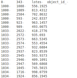
The code below save the gpm gpmdistance, created in section 3 in the file "gpmnetwork.GWT", presented in Figure 8.
More informations about the GAL and GWT formats can be found in the GeoDa User’s Guide and in the SpaceStat documentation.
| Num_attributes | Layer_1 | Layer_2 | Attribute_1 | Attribute_2 | ... | Attribute_N |
| ID_Object_1 | Num_Neighbors | |||||
| ID_Neighbor_1 | Attrib_1_Neigh_1 | Attrib_2_Neigh_1 | ... | Attrib_N_Neigh_1 | ID_Neighbor_2 | ... |
| ID_Object_2 | ... | |||||
| ... | ||||||
| 0 | Num_elements | Layer | Key_Variable |
| ID_Object_1 | Num_Neighbors | ||
| ID_Neighbor_1 | ID_Neighbor_2 | ... | ID_Neighbor_N |
| ... | |||