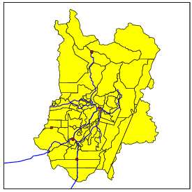
Figure 1: Points, lines, and polygons used in this vignette.
Fill cell functions calculate attribute values for tables associated with layers of cells. The goal is to homogenize information from different sources in different formats (vector data, rasters as well as other cellular layers), aggregating them into a single spatial (and possibly temporal) data source. Different operators are available according to the geometrical representation and semantics of the input data.
In the current TerraLib version, cells are rectangular. They may have a resolution of, for instance 1m x 1m, 500m x 500m, 100km x 200km, according to the application needs. A single cellular layer may be associated to different tables, which can be static (attributes that do not change over time) or dynamic (attributes that change over time).
To execute the steps in this tutorial, some spatial data is required:
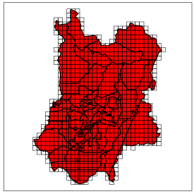
A layer of cells is created from another database layer. There are two strategies to create cells, depending on the type of spatial data of reference. The default way of creating cells is from layers of polygons. The code below creates the cells shown in Figure 2.
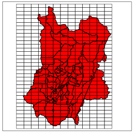
The default options create squared cells from the polygons. Bounding boxes of the whole set of polygonal geometries can also be used to create the layer of cells, using the argument all. In the next example, we create a layer of non-squared cells by informing different resolutions for x and y:
Cells created this way cover the entire area of bounding box covering the reference layer, similarly to a raster with a constant number of cells in each row and column. The result is shown in Figure 3. In both cases, a static table with the same name of the layer of cells is created automatically.
Cell attributes are created directly from the table of the layer of cells. The first step to fill cell attributes is to open the table:
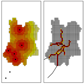
To create attributes using TerraLib functionalities, we use createAndFillColumn(). This function may take different arguments depending on the strategy used to fill the cells. The first argument is the table where the result will be stored, the second is the name of the attribute to be created, the third is the theme with the data used to compute the attribute, and the other depend on the operation. For example, if one wants to create an attribute based on the minimum distance from the centroid of the cells to a set of points, we can use strategy “distance”.
Operations such as distance may be used with any geometric type as parameter. However, some operations can be used with only one geometric type. For example, the length of lines covering each cell can be created by calling:
The results of these two operations are shown in Figure 4.
Some strategies use not only geometries but also attributes related to those geometries. To create an attribute that computes the maximum value of a given geometry that has some overlap with the cells just call:
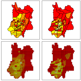
Table 1, in the end of this vignette, describes each operation available for filling cells directly from createAndFillColumn(). Most of the strategies are intuitive, but two deserve more attention, “sumwba” and “averagewba,” which mean “sum weighted by area” and “average weighted by area,” respectively. The first spreads a given attribute of a set of polygons through the cells. This operation can be used for population data, because it keeps the overall sum of the data in both sets. The second operation if useful to work with attributes representing averages. The algorithm spreads averages of a set of polygons to the cells, recomputing each average proportionally to the intersection area. The results of these operations are shown in Figure 5.
Finally, to visualize the data it is necessary to create a theme using the table that contains the attributes created.
The figures plotted in this vignette use plotColoured(), described and used as follows:
Aditionally, it is possible to create new attributes directly using createColumn() and updateColumns(), instead of createAndFillColumn(). This way, you can use all R functionalities to generate attributes according to the objectives of the work. For further information on how to create attributes of tables, read the vignette “Tables and Queries With aRT,” available within the package.
| Operation | Description |
| area | Total area of overlay between the cell and a layer of polygons. |
| average | Average of an attribute of the objects that have some intersection with the cell, without taking into account their geometric properties. |
| averagewba | Average weighted by area, based on the proportion of the intersection area. Useful when you want to distribute atributes that represent averages, such as per capita income. |
| count | Number of objects that have some overlay with the cell (requires argument geometry). |
| distance | Distance to the nearest object of a chosen geometry (requires argument geometry). |
| length | Total length of overlay between the cell and a layer of lines. |
| majority | More common value in the objects that have some intersection with the cell, without taking into account their geometric properties. |
| maximum | Maximum value of an attribute among the objects that have some intersection with the cell, without taking into account their geometric properties. |
| minimum | Minimum value of an attribute among the objects that have some intersection with the cell, without taking into account their geometric properties. |
| percentage | Percentages of each class of a raster data. It creates one attribute for each class of the raster. |
| presence | Boolean value pointing out whether some object has an overlay with the cell. |
| stdev | Standard deviation of an attribute of the objects that have some intersection with the cell, without taking into account their geometric properties. |
| sum | Sum of an attribute of the objects that have some intersection with the cell, without taking into account their geometric properties. |
| sumwba | Sum weighted by area, based on the proportion of the intersection area. Useful when you want to preserve the total amount in both layers, such as population size. |
| xdistance | Approximated distance to the nearest object of a chosen geometry (requires arguments geometry and maxerror). |